bfrr

Calculate Bayes Factors and robustness regions from summary statistics.

Installation

You can install the development version from GitHub with:

# install.packages("devtools")
devtools::install_github("debruine/bfrr")

Example

library(bfrr)
library(ggplot2)
library(cowplot)

First, we’ll simulate 50 data points from a normal distribution with a mean of 0.25 and SD of 1 and conduct a one-sample t-test.

simdat <- rnorm(50, 0.25, 1)
t.test(simdat)
#> 
#>  One Sample t-test
#> 
#> data:  simdat
#> t = 2.9009, df = 49, p-value = 0.005558
#> alternative hypothesis: true mean is not equal to 0
#> 95 percent confidence interval:
#>  0.1083681 0.5970156
#> sample estimates:
#> mean of x 
#> 0.3526918

Set up the test using bfrr().

rr <- bfrr(
  sample_mean = mean(simdat), # mean of the sample
  sample_se = sd(simdat) / sqrt(length(simdat)), # SE of the sample
  sample_df = length(simdat) - 1, # degrees of freedom
  model = "normal",
  mean = 0, # mean of the H1 distribution
  sd = 0.25, # SD of the H1 distribution
  tail = 1, # is the test 1-tailed or 2-tailed
  criterion = 6, # BF against which to test for support for H1/H0
  rr_interval = list( # ranges to vary H1 parameters for robustness regions
    mean = c(-2, 2), # explore H1 means from 0 to 2
    sd = c(0, 2) # explore H1 SDs from 0 to 2
  ),
  precision = 0.05 # precision to vary RR parameters
)

Use summary(rr) to output a summary paragraph.

summary(rr)

The likelihood of your data under the theoretical distribution N(0, 0.25) is 0.16. The likelihood of your data under the null distribution T(49) is 0.01. The Bayes Factor is 20.6; this test finds evidence for H1 with a criterion of 6. The region of theoretical model parameters that give the same conclusion is HN([-0.2, 0.9], 0.25); HN(0, [0.1, 2]).

Use plot(rr) to view a plot of your data.

plot(rr)

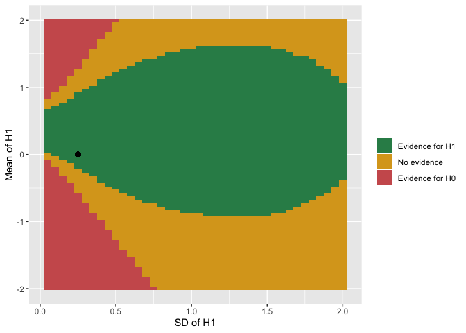
If your mean is 0 or you set the same number for the lower and upper bounds of a parameter’s rr_interval, that parameter won’t vary and you’ll get a graph that looks like this.

r1 <- bfrr(sample_mean = 0.25, tail = 1)
r2 <- bfrr(sample_mean = 0.25, tail = 2)
p1 <- plot(r1)
p2 <- plot(r2)

p1t <- paste0("One-tailed H1, RR = [", toString(r1$RR$sd), "]")
p2t <- paste0("Two-tailed H1, RR = [", toString(r2$RR$sd), "]")
cowplot::plot_grid(p1 + ggtitle(p1t), 
                   p2 + ggtitle(p2t), 
                   nrow = 2)