Simulate from Existing Data

library(ggplot2)
library(dplyr)
library(tidyr)
library(faux)

The sim_df() function produces a data table with the same distributions and correlations as an existing data table. It simulates all numeric variables from a continuous normal distribution (for now).

For example, here is the relationship between speed and distance in the built-in dataset cars.

cars %>%
  ggplot(aes(speed, dist)) + 
  geom_point() +
  geom_smooth(method = "lm", formula = "y~x")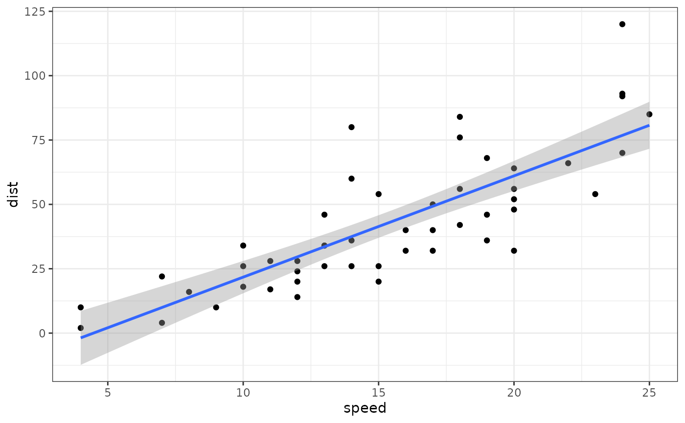

Original cars dataset

You can create a new sample with the same parameters and 500 rows with the code sim_df(cars, 500).

sim_df(cars, 500) %>%
  ggplot(aes(speed, dist)) + 
    geom_point() +
    geom_smooth(method = "lm", formula = "y~x")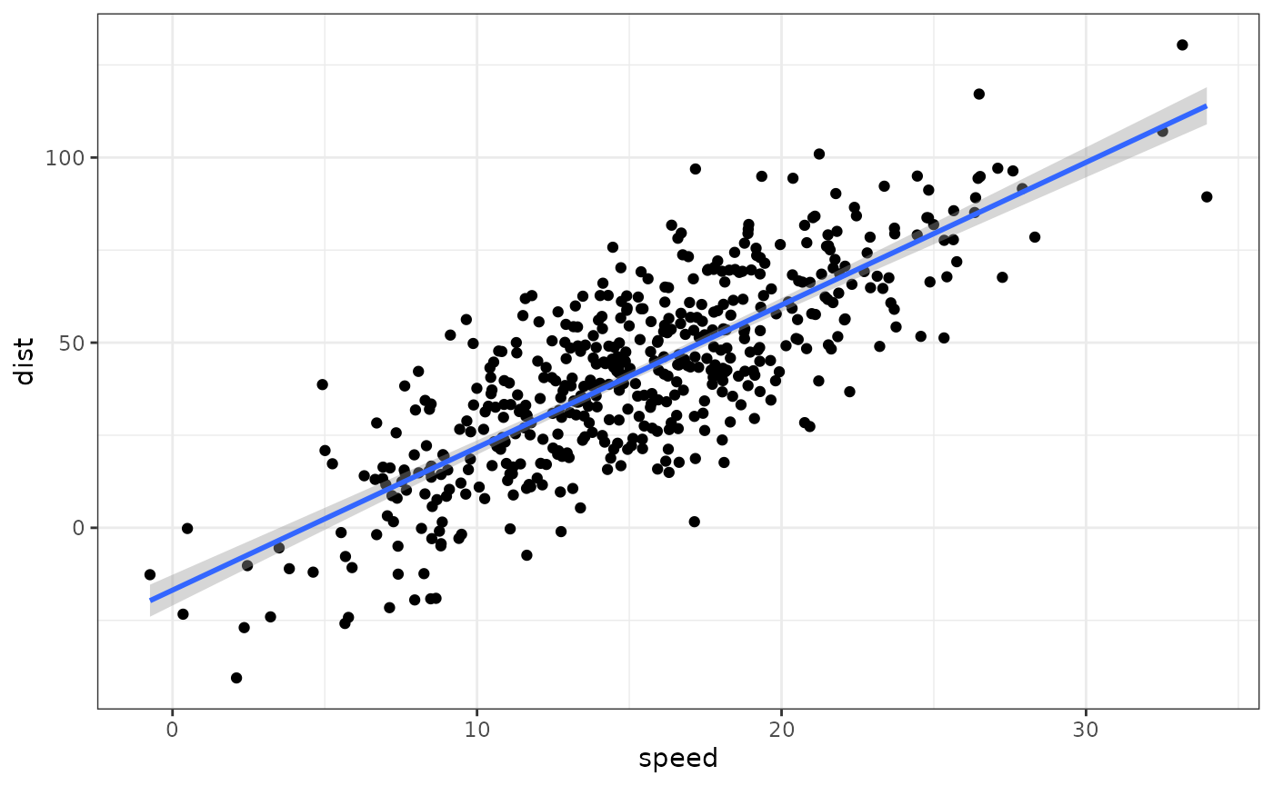

Simulated cars dataset

Between-subject variables

You can also optionally add between-subject variables. For example, here is the relationship between horsepower (hp) and weight (wt) for automatic (am = 0) versus manual (am = 1) transmission in the built-in dataset mtcars.

mtcars %>%
  mutate(transmission = factor(am, labels = c("automatic", "manual"))) %>%
  ggplot(aes(hp, wt, color = transmission)) +
  geom_point() +
  geom_smooth(method = "lm", formula = "y~x")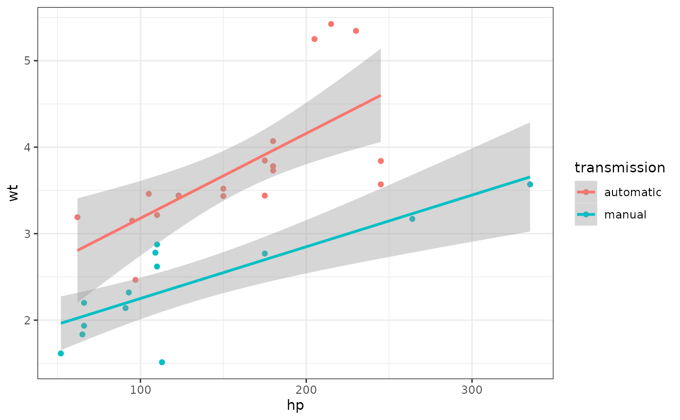

Original mtcars dataset

And here is a new sample with 50 observations of each.

sim_df(mtcars, 50 , between = "am") %>%
  mutate(transmission = factor(am, labels = c("automatic", "manual"))) %>%
  ggplot(aes(hp, wt, color = transmission)) +
  geom_point() +
  geom_smooth(method = "lm", formula = "y~x")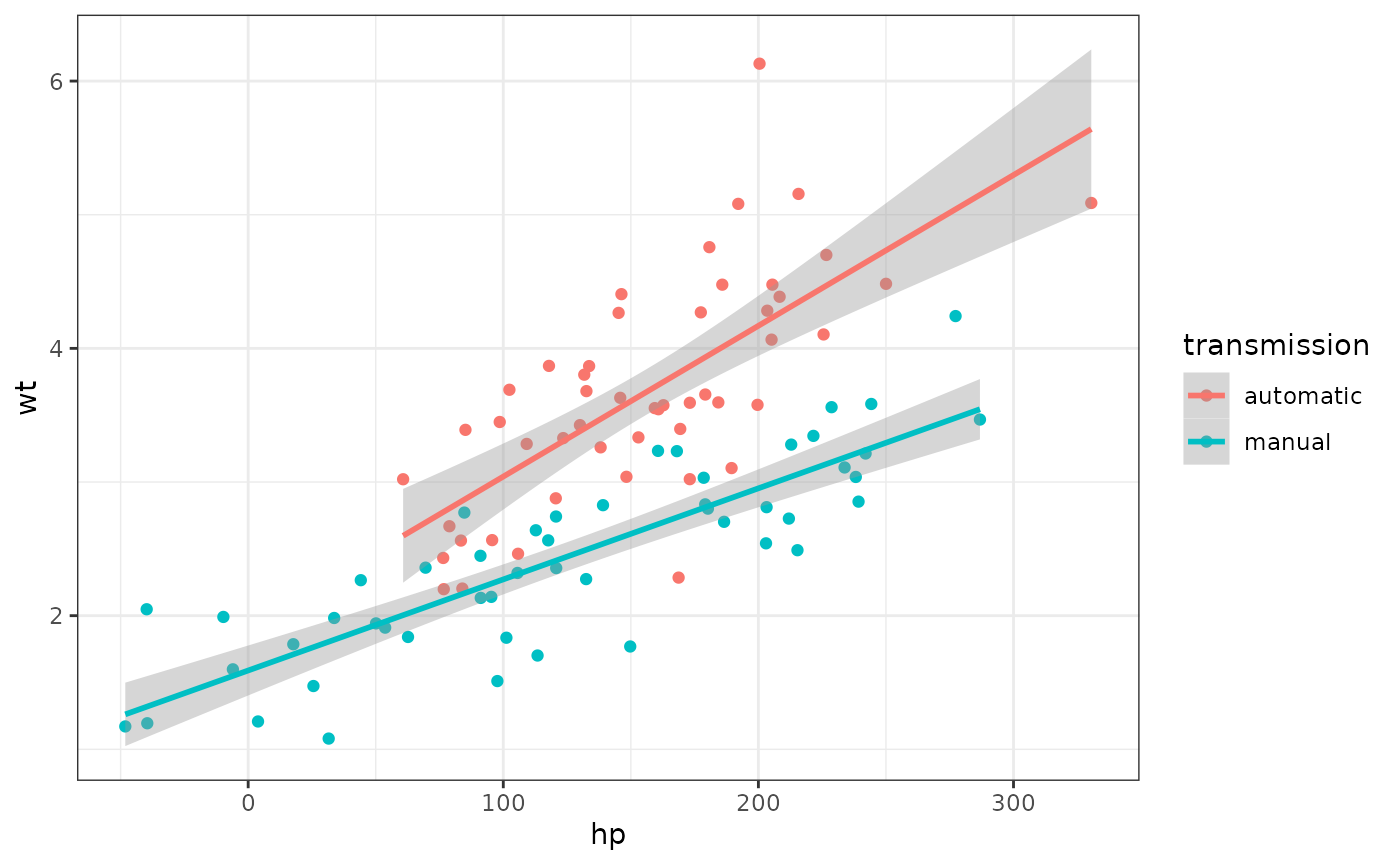

Simulated iris dataset

Empirical

Set empirical = TRUE to return a data frame with exactly the same means, SDs, and correlations as the original dataset.

exact_mtcars <- sim_df(mtcars, 50, between = "am", empirical = TRUE)

Rounding

For now, the function only creates new variables sampled from a continuous normal distribution. I hope to add in other sampling distributions in the future. So you’d need to do any rounding or truncating yourself.

sim_df(mtcars, 50, between = "am") %>%
  mutate(hp = round(hp),
         transmission = factor(am, labels = c("automatic", "manual"))) %>%
  ggplot(aes(hp, wt, color = transmission)) +
  geom_point() +
  geom_smooth(method = "lm", formula = "y~x")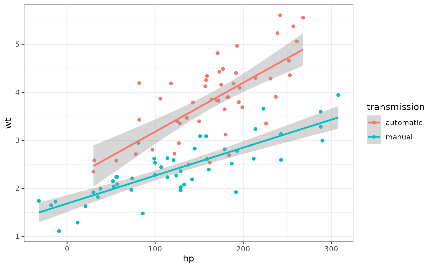

Simulated iris dataset (rounded)

Missing data

As of faux 0.0.1.8, if you want to simulate missing data, set missing = TRUE and sim_df will simulate missing data with the same joint probabilities as your data. In the dataset below, in condition B1a, 30% of W1a values are missing and 60% of W1b values are missing. This is correlated so that there is a 100% chance that W1b is missing if W1a is. There is no missing data for condition B1b.

data <- sim_design(2, 2, n = 10, plot = FALSE)
data$W1a[1:3] <- NA
data$W1b[1:6] <- NA
data
#>     id  B1         W1a         W1b
#> 1  S01 B1a          NA          NA
#> 2  S02 B1a          NA          NA
#> 3  S03 B1a          NA          NA
#> 4  S04 B1a -0.87577954          NA
#> 5  S05 B1a  0.27931928          NA
#> 6  S06 B1a  0.46277729          NA
#> 7  S07 B1a -0.11678369 -0.66795544
#> 8  S08 B1a  1.34454748  2.30398889
#> 9  S09 B1a -1.26771349  0.55738252
#> 10 S10 B1a -0.71258675  0.09183975
#> 11 S11 B1b -0.39607245  0.85023624
#> 12 S12 B1b -1.15357665 -0.18013489
#> 13 S13 B1b -0.21533313  1.08873598
#> 14 S14 B1b -0.42370435  0.94812875
#> 15 S15 B1b -0.05717782  0.63667947
#> 16 S16 B1b -0.12733224 -1.47331528
#> 17 S17 B1b  0.21208884  0.69005635
#> 18 S18 B1b -0.20401676 -1.01059002
#> 19 S19 B1b -1.14885697 -0.50127757
#> 20 S20 B1b  0.87586766  1.47606428

The simulated data will have the same pattern of missingness (sampled from the joint distribution, so it won’t be exact).

simdat <- sim_df(data, between = "B1", n = 1000, 
                 missing = TRUE)

B1	W1a	W1b	n
B1a	NA	NA	0.31
B1a	not NA	NA	0.31
B1a	not NA	not NA	0.38
B1b	not NA	not NA	1.00

Lisa DeBruine

2023-09-24

Between-subject variables

Empirical

Rounding

Missing data