Why Code?

https://debruine.github.io/why-code

Lisa DeBruine

Abstract

Research transparency and integrity benefit greatly from computationally reproducible code, but the barriers to learning the required skills can seem overwhelming. In this talk, I will summarise the benefits of using code to process and analyse data, give some practical tips for developing your skills, demonstrate how data simulation can improve your research, and discuss the benefits of code review.

Why Use Code?

Plots!

UN Population Data

Location	Sex	Age	1950	1955	1960	1965	1970	1975	1980	1985	1990	1995	2000	2005	2010	2015	2020	2025	2030	2035	2040	2045	2050	2055	2060	2065	2070	2075	2080	2085	2090	2095	2100
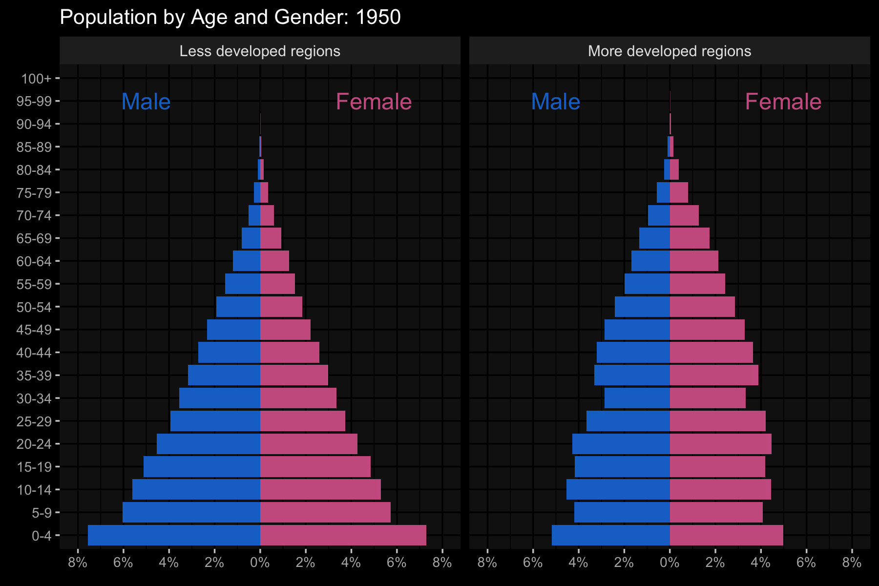
More developed regions	Both sexes combined	0-4	82893	87593	89475	87953	82992	81473	78083	78191	77564	71194	65679	65933	69648	69387	67495	65329	63693	62957	63263	63749	63609	62818	61897	61280	61143	61301	61426	61290	60905	60494	60264
More developed regions	Female	0-4	40614	42827	43734	42969	40569	39787	38068	38175	37841	34704	32011	32135	33942	33801	32889	31839	31043	30683	30831	31066	30997	30613	30166	29867	29800	29877	29938	29873	29686	29487	29376
More developed regions	Male	0-4	42279	44766	45740	44984	42423	41686	40015	40016	39723	36490	33667	33797	35706	35586	34606	33490	32650	32274	32432	32683	32611	32205	31731	31414	31343	31424	31488	31417	31219	31007	30888
Less developed regions	Both sexes combined	0-4	255604	319584	344533	391350	441088	463037	469514	511937	565990	548648	549987	561305	582366	601287	610447	611590	613750	618254	622382	625782	626567	625214	621668	617656	612496	606880	600527	592475	583450	573573	563352
Less developed regions	Female	0-4	125463	156409	168668	191349	216219	226435	229366	249556	275064	265413	265513	270549	280889	290626	295620	296746	298526	301376	303650	305531	305977	305360	303662	301729	299227	296489	293381	289435	285012	280171	275160
Less developed regions	Male	0-4	130141	163175	175866	200001	224870	236603	240149	262381	290926	283235	284474	290757	301478	310661	314827	314844	315224	316878	318732	320251	320590	319854	318006	315928	313269	310390	307147	303040	298438	293402	288193

UN Population Data: 2020

sex	year	age	pop	pcnt
Female	2020	0-4	328509	4.21%
Female	2020	5-9	321512	4.12%
Female	2020	10-14	309770	3.97%
Female	2020	15-19	295553	3.79%
Female	2020	20-24	289101	3.71%
Female	2020	25-29	288633	3.70%
Female	2020	30-34	296294	3.80%
Female	2020	35-39	268372	3.44%
Female	2020	40-44	244400	3.14%
Female	2020	45-49	238134	3.06%
Female	2020	50-54	223163	2.86%
Female	2020	55-59	195634	2.51%
Female	2020	60-64	164961	2.12%
Female	2020	65-69	140704	1.81%

sex	year	age	pop	pcnt
Female	2020	70-74	101491	1.30%
Female	2020	75-79	69027	0.89%
Female	2020	80-84	48282	0.62%
Female	2020	85-89	26429	0.34%
Female	2020	90-94	11352	0.15%
Female	2020	95-99	3056	0.04%
Female	2020	100+	449	0.01%
Male	2020	0-4	349433	4.48%
Male	2020	5-9	342927	4.40%
Male	2020	10-14	331497	4.25%
Male	2020	15-19	316643	4.06%
Male	2020	20-24	308287	3.96%
Male	2020	25-29	306060	3.93%
Male	2020	30-34	309237	3.97%

sex	year	age	pop	pcnt
Male	2020	35-39	276447	3.55%
Male	2020	40-44	249389	3.20%
Male	2020	45-49	241233	3.09%
Male	2020	50-54	222610	2.86%
Male	2020	55-59	192215	2.47%
Male	2020	60-64	157180	2.02%
Male	2020	65-69	128939	1.65%
Male	2020	70-74	87186	1.12%
Male	2020	75-79	54755	0.70%
Male	2020	80-84	33649	0.43%
Male	2020	85-89	15757	0.20%
Male	2020	90-94	5328	0.07%
Male	2020	95-99	1078	0.01%
Male	2020	100+	124	0.00%

Set up plot

ggplot(data = pop_data_2020, 
       mapping = aes(x = age, y = pcnt, fill = sex))

Add visualistion

ggplot(pop_data_2020, aes(age, pcnt, fill = sex)) +
  geom_col()

Flip the x and y axes

ggplot(pop_data_2020, aes(age, pcnt, fill = sex)) +
  geom_col() +
  coord_flip()

Center the columns

pop_data_2020 <- pop_data_2020 |>
  mutate(pcnt2 = ifelse(sex == "Male", -pcnt, pcnt))

ggplot(pop_data_2020, aes(age, pcnt2, fill = sex)) +
  geom_col() +
  coord_flip()

Fix the titles

ggplot(pop_data_2020, aes(age, pcnt2, fill = sex)) +
  geom_col() +
  coord_flip() +
  labs(title = "Population by Age and Gender: 2020",
       x = "Age", y = "Percent of Population")

Remove legend

ggplot(pop_data_2020, aes(age, pcnt2, fill = sex)) +
  geom_col(show.legend = FALSE) +
  coord_flip() +
  labs(title = "Population by Age and Gender: 2020",
       x = "Age", y = "Percent of Population")

Customise colours

ggplot(pop_data_2020, aes(age, pcnt2, fill = sex)) +
  geom_col(show.legend = FALSE) +
  coord_flip() +
  labs(title = "Population by Age and Gender: 2020",
       x = "Age", y = "Percent of Population") +
  scale_fill_manual(
    values = c("hotpink3", "dodgerblue3"))

Customise the axes

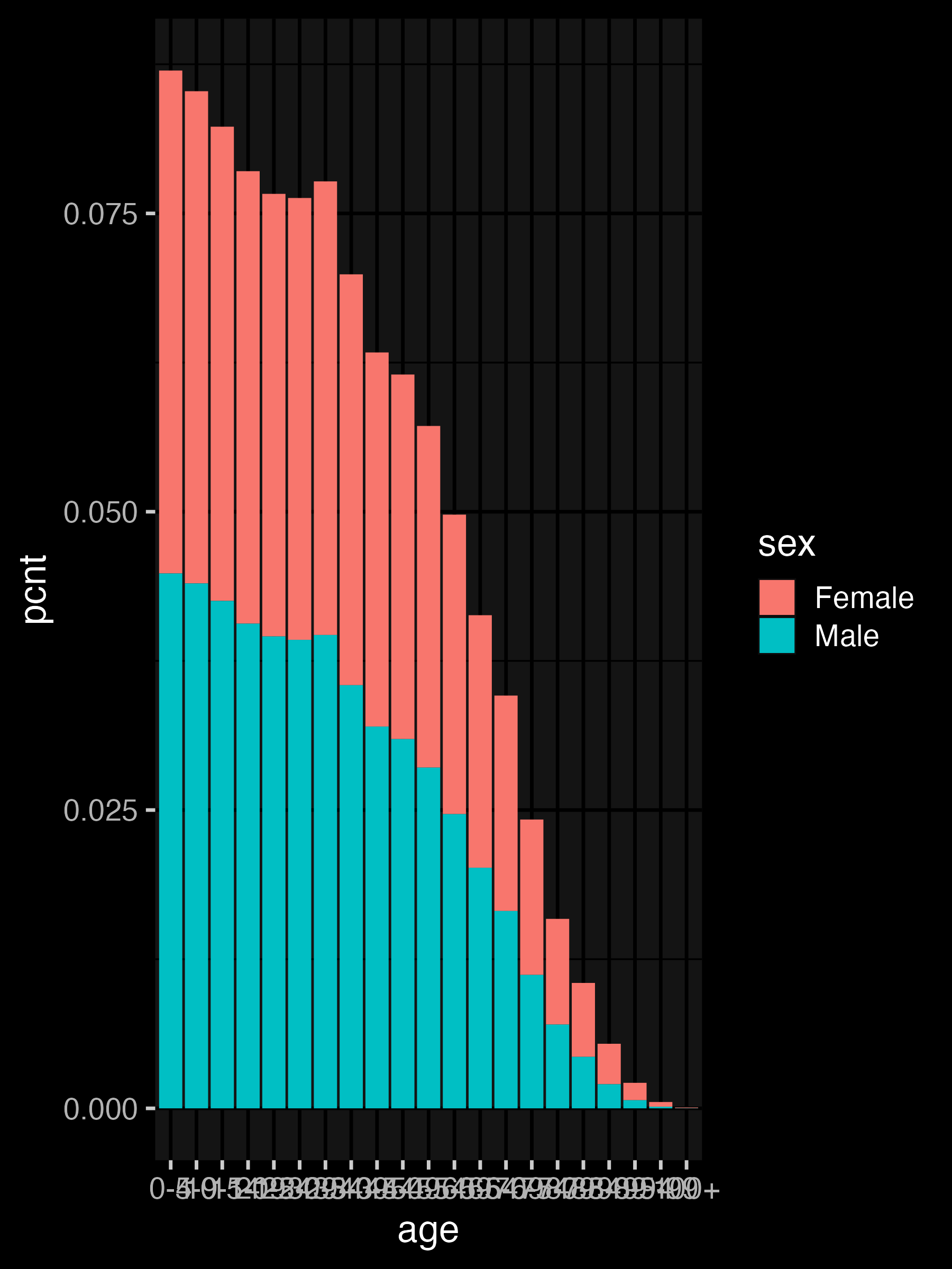
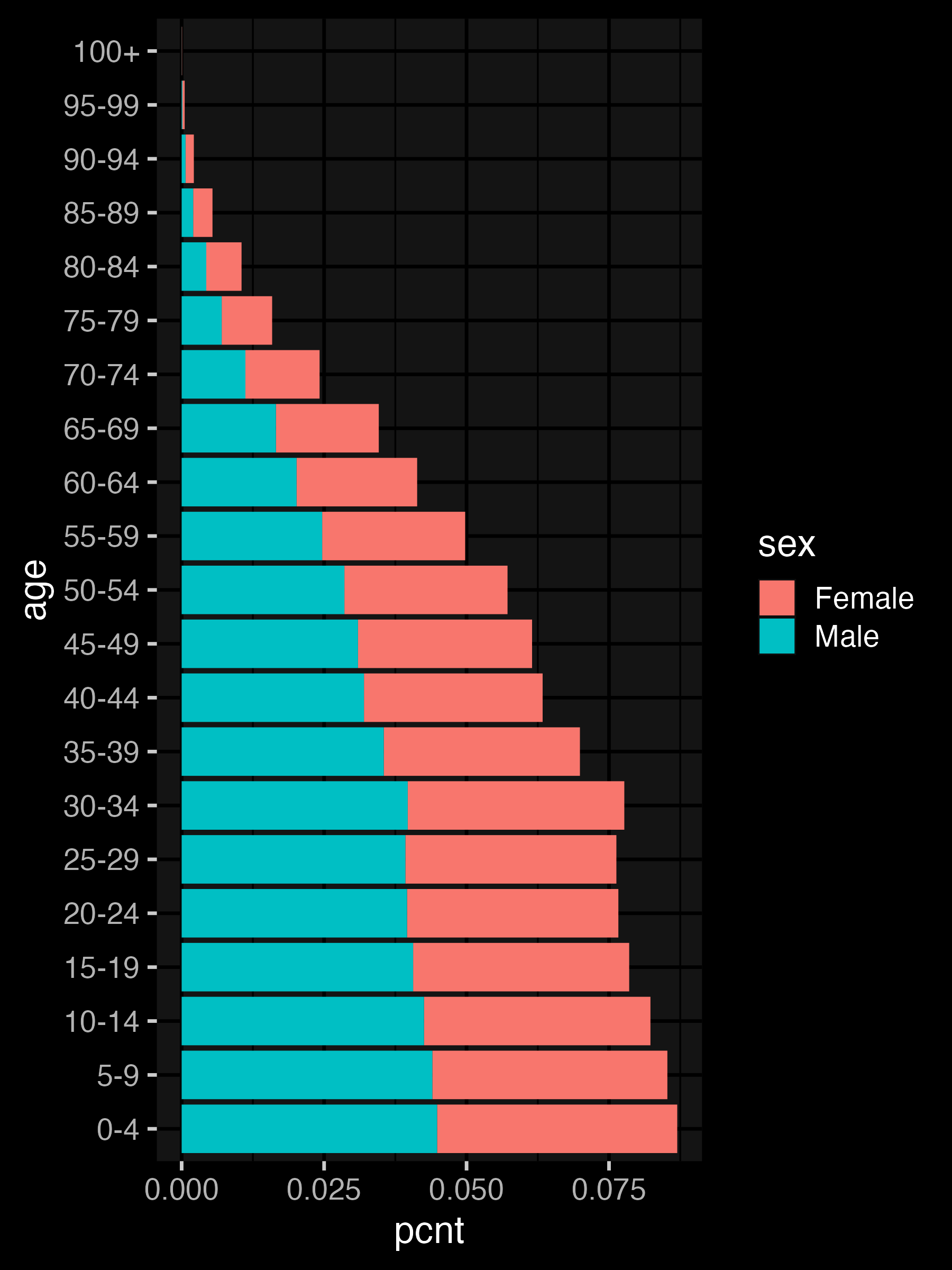
ggplot(pop_data_2020, aes(age, pcnt2, fill = sex)) +
  geom_col(show.legend = FALSE) +
  coord_flip() +
  labs(title = "Population by Age and Gender: 2020",
       x = "Age", y = "Percent of Population") +
  scale_fill_manual(
    values = c("hotpink3", "dodgerblue3")) +
  scale_y_continuous(
    breaks = seq(-.04, .04, .01),
    labels = abs(seq(-4, 4, 1)) |> paste0("%"))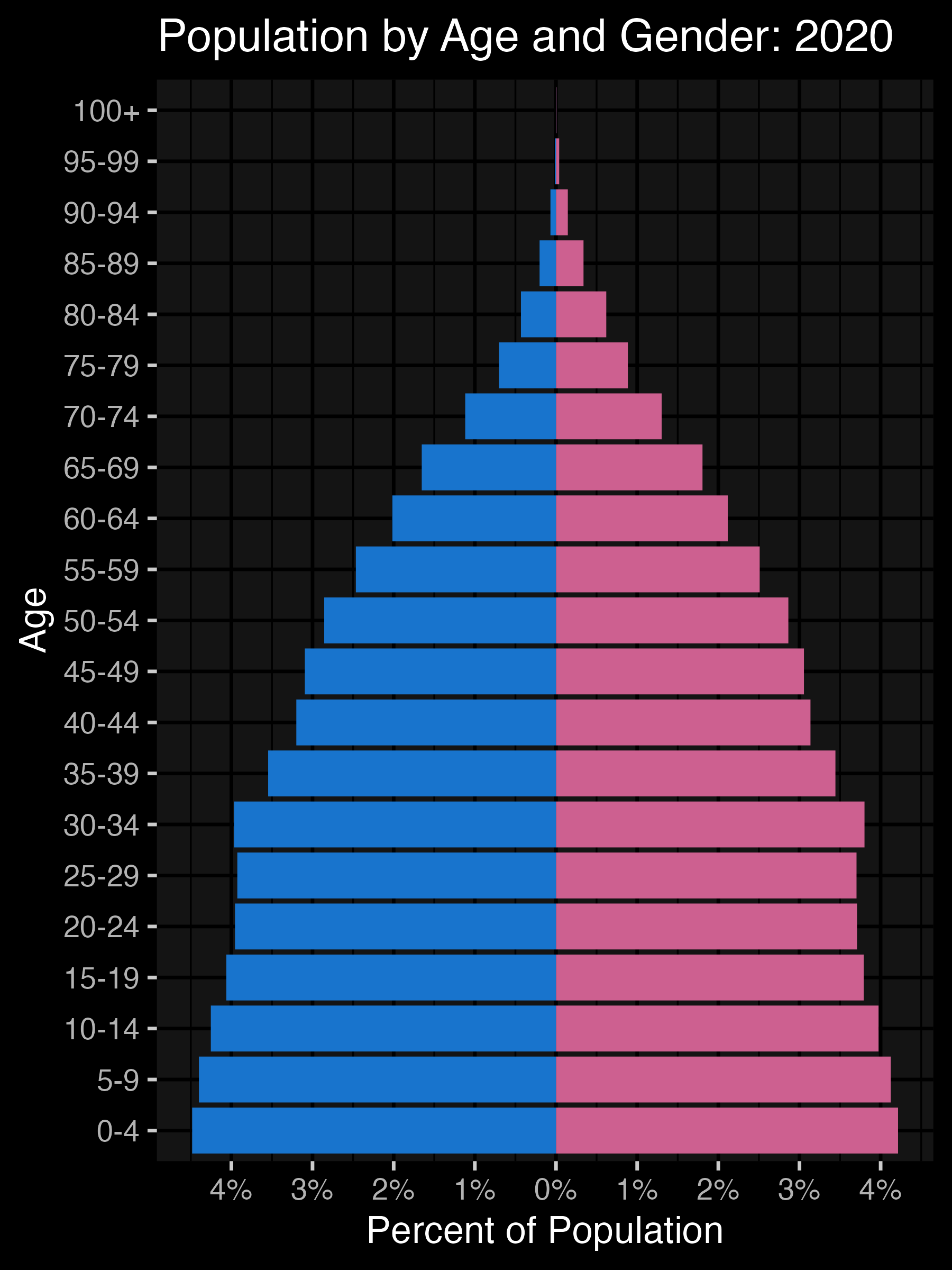

Add annotations

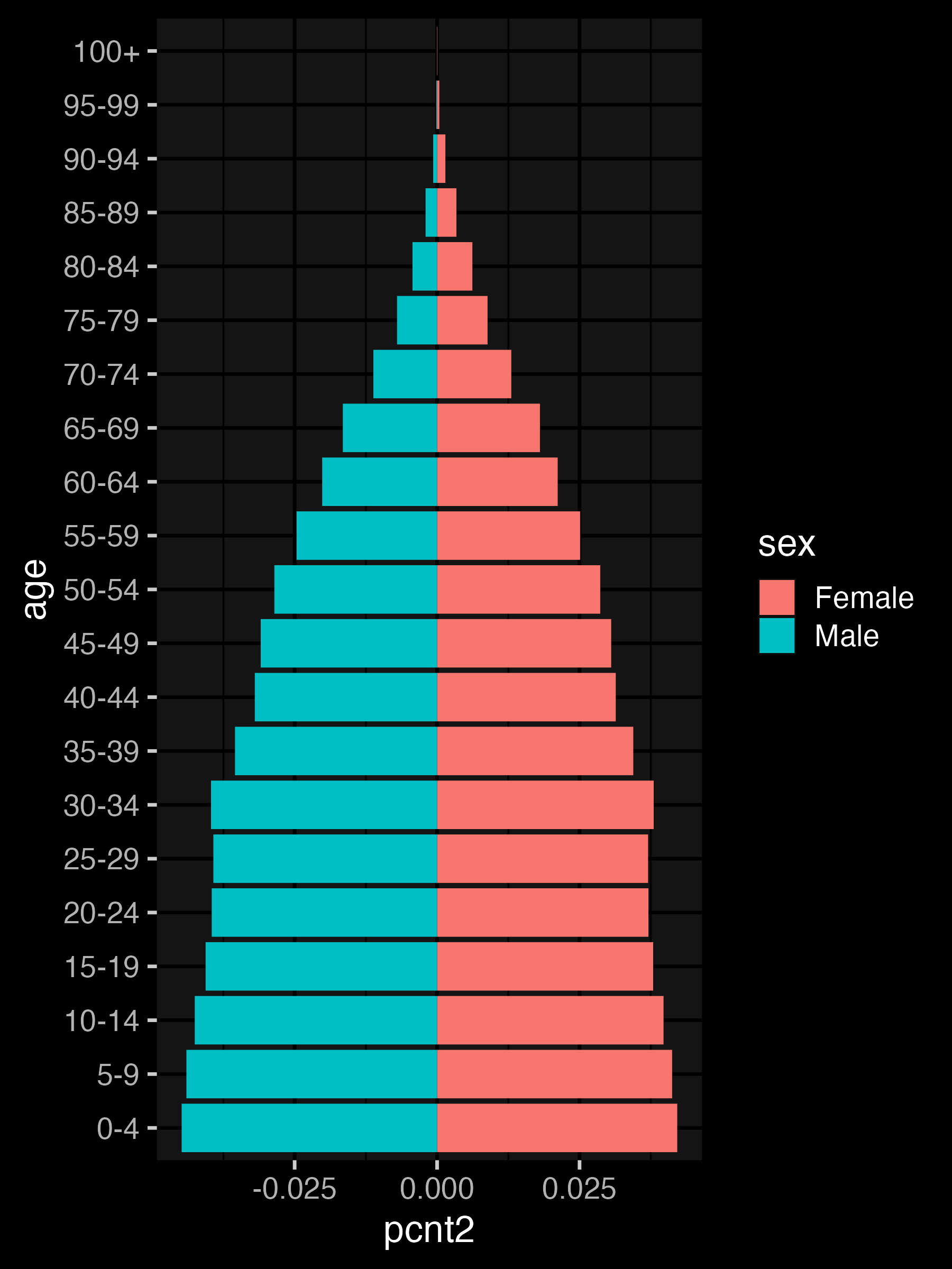
ggplot(pop_data_2020, aes(age, pcnt2, fill = sex)) +
  geom_col(show.legend = FALSE) +
  coord_flip() +
  labs(title = "Population by Age and Gender: 2020",
       x = "Age", y = "Percent of Population") +
  scale_fill_manual(
    values = c("hotpink3", "dodgerblue3")) +
  scale_y_continuous(
    breaks = seq(-.04, .04, .01),
    labels = abs(seq(-4, 4, 1)) |> paste0("%")) +
  annotate("text", label = "Female", size = 8, 
    color = "hotpink3", x = 20, y = .025) +
  annotate("text", label = "Male", size = 8, 
    color = "dodgerblue3", x = 20, y = -.025)

Animate

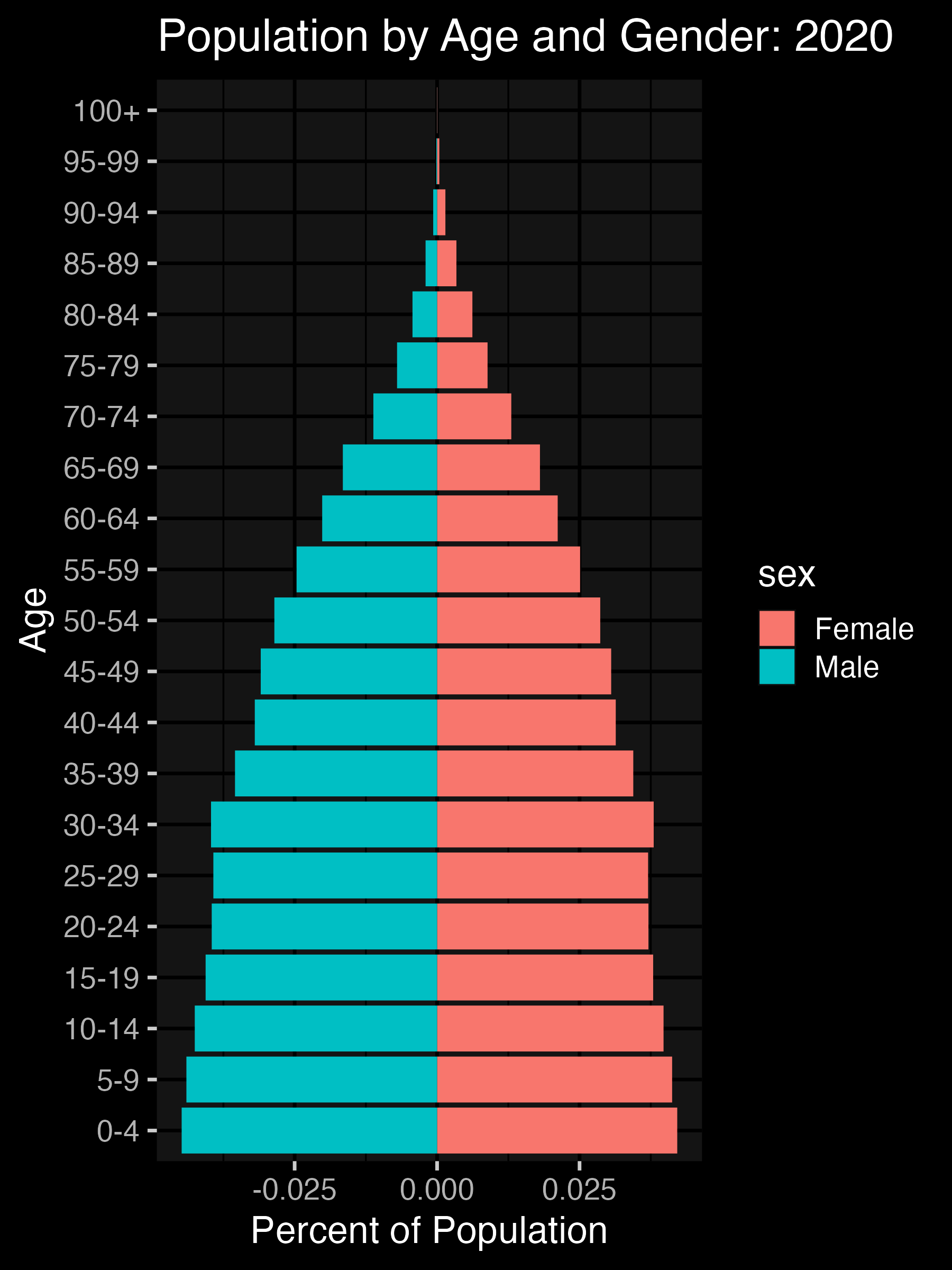
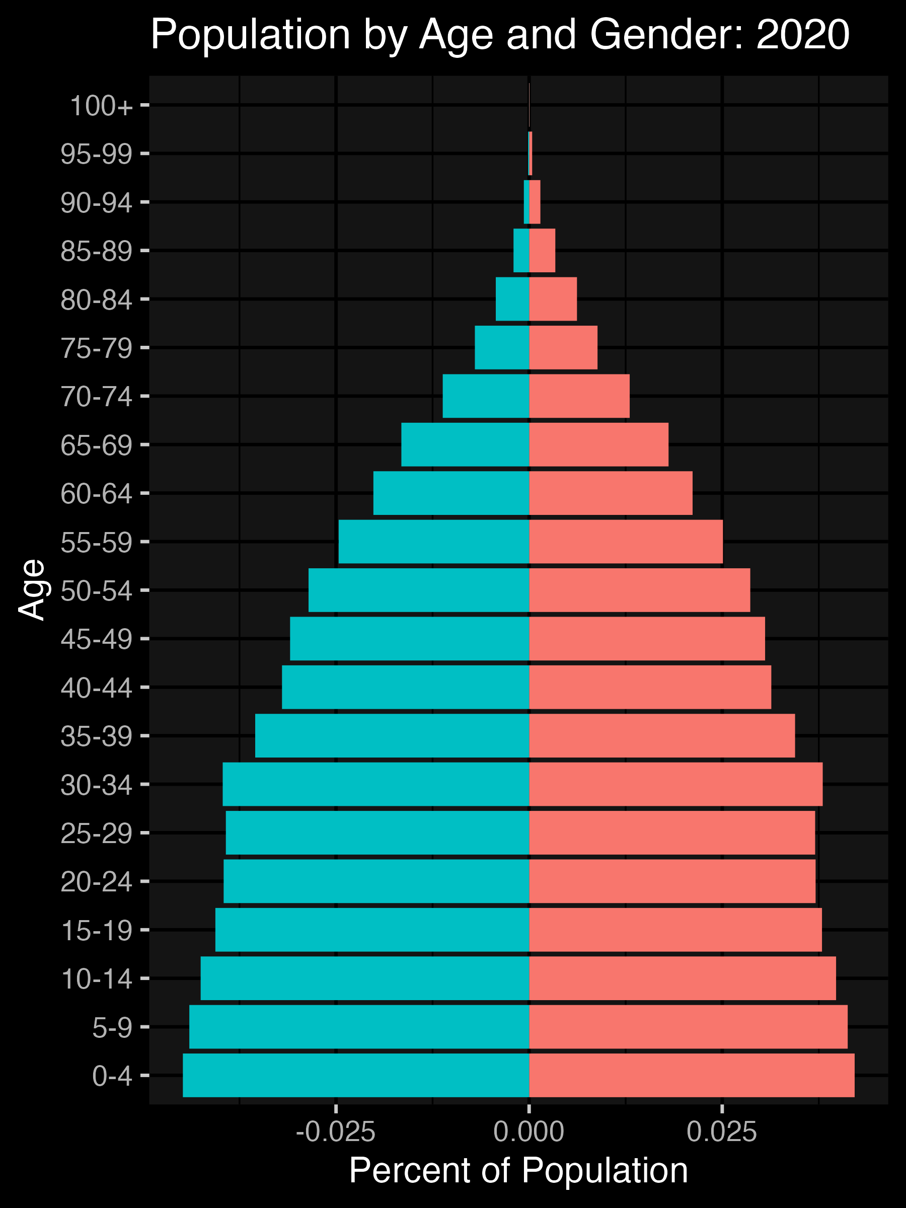
ggplot(pop_data, aes(age, pcnt2, fill = sex)) +
  geom_col(show.legend = FALSE) +
  coord_flip(ylim = c(-.08, .08)) +
  labs(title = "Population by Age and Gender: 
                {floor(frame_time/5)*5}",
       x = "Age", y = "Percent of Population") +
  scale_fill_manual(
    values = c("hotpink3", "dodgerblue3")) +
  scale_y_continuous(
    breaks = seq(-.08, .08, .02),
    labels = abs(seq(-8, 8, 2)) |> paste0("%")) +
  annotate("text", label = "Female", size = 8, 
    color = "hotpink3", x = 20, y = .05) +
  annotate("text", label = "Male", size = 8, 
    color = "dodgerblue3", x = 20, y = -.05) +
  gganimate::transition_time(year)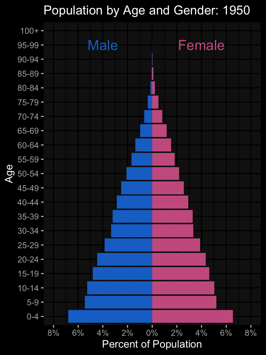

Reusability

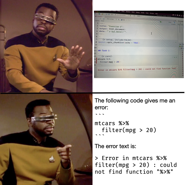
Error Detection

An analysis by Nuijten et al. (2016) of over 250K p-values reported in 8 major psych journals from 1985 to 2013 found that:

half the papers had at least one inconsistent p-value
1/8 of papers had errors that could affect conclusions
errors more likely to be erroneously significant than not

Computational Reproducibility

Of 35 articles published in Cognition with usable data (but no code, Hardwicke et al. (2018) found:
- only 11 could be reproduced independently
- 11 were reproducible with the original authors’ help
- 13 were not reproducible even by the original authors
Of 62 psych Registered Reports published from 2014–2018, 37 had analysis scripts, 31 could be run, and 21 reproduced all the main results (Obels et al, 2020)

Developing Skills

Top Tips

Take a workshop in your area
Practice regularly and meaningfully
Embed R in your daily practice
Do something fun!

PsyTeachR

Data Visualisation Using R, for Researchers Who Don’t Use R

Learning Statistical Models Through Simulation in R

Online Communities

#RStats mastodon

#RStats twitter

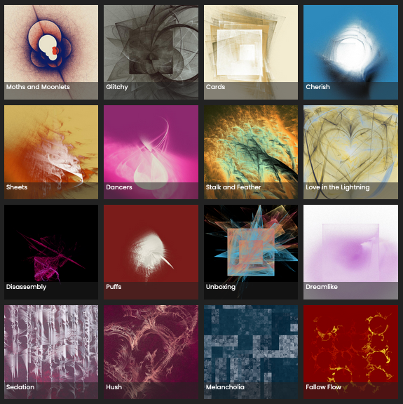
Art and Memes

RStats Musical Memes @rafa_moral

It’s R! 🌽

Dirtbag 👶

Data 😱

Data Simulation

Uses for Data Simulation

Being able to simulate data allows you to:

prep analysis scripts for pre-registration
calculate power and sensitivity for analyses that don’t have empirical methods
create reproducible examples when your data are too big or confidential to share
enhance your understanding of statistical concepts
create demo data for teaching and tutorials

Faux Code

sim_data <- faux::sim_design(
  within = list(version = c(V1 = "Version 1", V2 = "Version 2"), 
                condition = c(ctl = "Control", exp = "Experimental")),
  between = list(age_group = c(young = "Age 20-29", old = "Age 70-79")),
  n = 30,
  mu = c(100, 100, 100, 100, 100, 90, 110, 110),
  sd = 20,
  r = 0.5,
  dv = c(score = "Score"),
  id = c(id = "Subject ID"),
  vardesc = list(version = "Task Version", 
                 condition = "Experiment Condition", 
                 age_group = "Age Group"),
  long = TRUE
)

Faux Design Parameters

age_group	version	condition	V1_ctl	V1_exp	V2_ctl	V2_exp	n	mu	sd
young	V1	ctl	1.0	0.5	0.5	0.5	30	100	20
young	V1	exp	0.5	1.0	0.5	0.5	30	100	20
young	V2	ctl	0.5	0.5	1.0	0.5	30	100	20
young	V2	exp	0.5	0.5	0.5	1.0	30	100	20
old	V1	ctl	1.0	0.5	0.5	0.5	30	100	20
old	V1	exp	0.5	1.0	0.5	0.5	30	90	20
old	V2	ctl	0.5	0.5	1.0	0.5	30	110	20
old	V2	exp	0.5	0.5	0.5	1.0	30	110	20

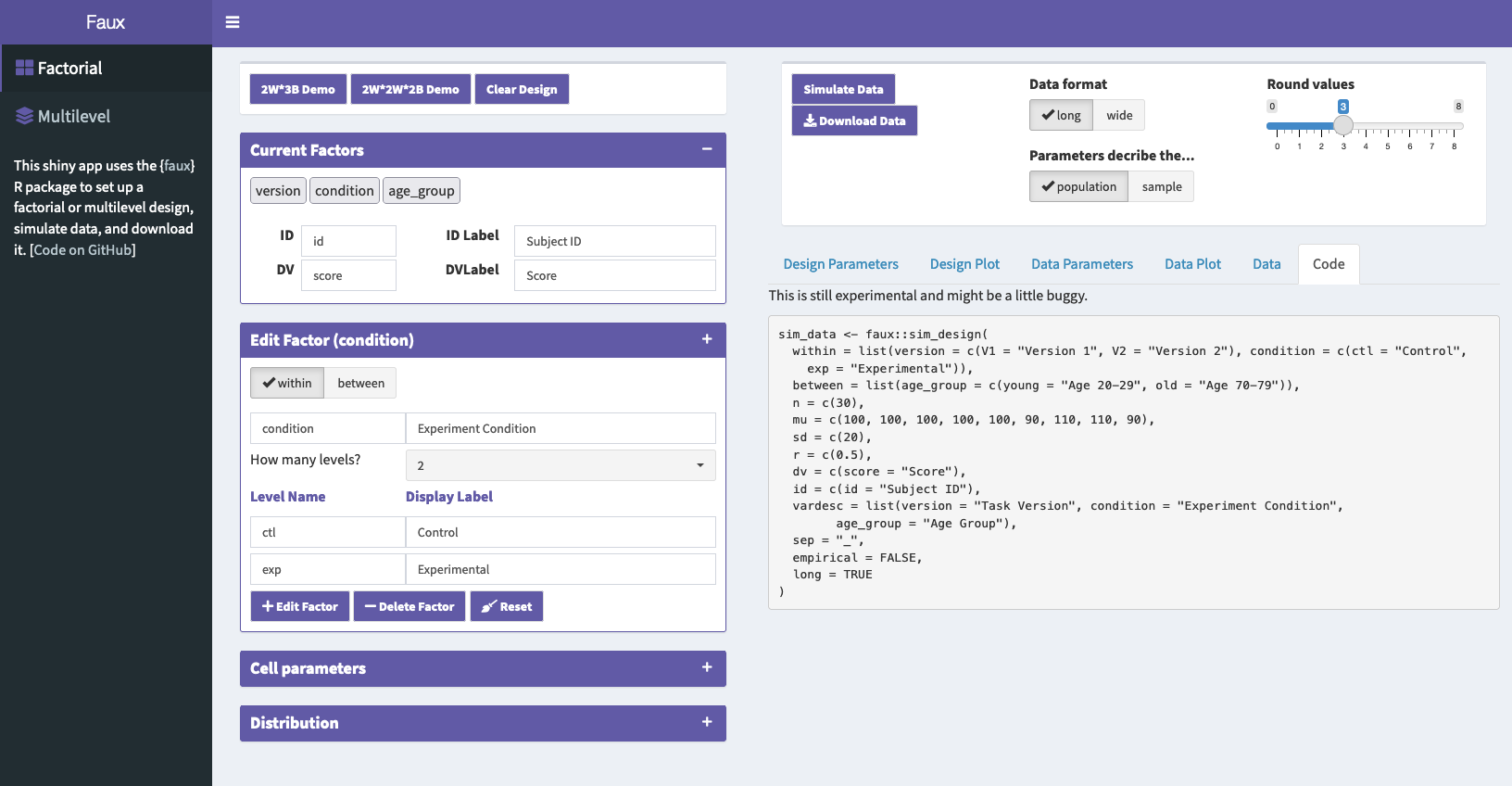
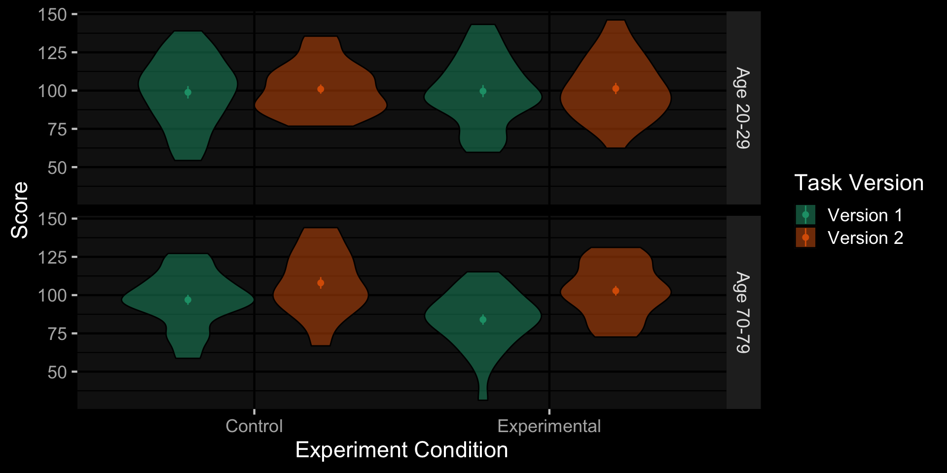
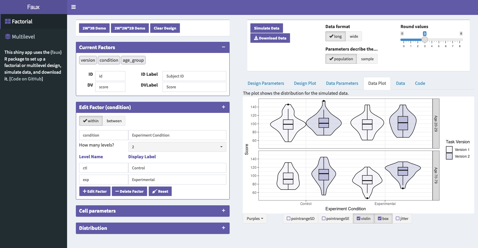
Faux Design Plot

Faux Data Plot

Power Simulation: Replicate Data

sim_data <- faux::sim_design(
  within = list(version = c(V1 = "Version 1", V2 = "Version 2"), 
                condition = c(ctl = "Control", exp = "Experimental")),
  between = list(age_group = c(young = "Age 20-29", old = "Age 70-79")),
  n = 30,
  mu = c(100, 100, 100, 100, 100, 90, 110, 110),
  sd = 20,
  r = 0.5,
  dv = c(score = "Score"),
  id = c(id = "Subject ID"),
  vardesc = list(version = "Task Version", 
                 condition = "Experiment Condition", 
                 age_group = "Age Group"),
  long = TRUE,
  rep = 100
)

Power Simulation: Analysis Function

# setup options to avoid annoying afex message & run faster
afex::set_sum_contrasts()
afex::afex_options(include_aov = FALSE) 

analysis <- function(data) {
  a <- afex::aov_ez(
    id = "id", 
    dv = "score", 
    between = "age_group",
    within = c("version", "condition"),
    data = data)
  
  as_tibble(a$anova_table, rownames = "term") |>
    rename(p = `Pr(>F)`)
}

Power Simulation: Analysis Result

# test on first data set
analysis(sim_data$data[[1]])

term	num Df	den Df	MSE	F	ges	p
age_group	1	58	845.2	0.50	0.005	0.480
version	1	58	215.9	28.56	0.069	0.000
age_group:version	1	58	215.9	14.90	0.037	0.000
condition	1	58	192.6	0.07	0.000	0.792
age_group:condition	1	58	192.6	4.89	0.011	0.031
version:condition	1	58	183.8	8.97	0.019	0.004
age_group:version:condition	1	58	183.8	0.30	0.001	0.587

Power Simulation

power <- sim_data |>
  mutate(analysis = purrr::map(data, analysis)) |>
  select(-data) |>
  unnest(analysis) |>
  group_by(term) |>
  summarise(power = mean(p < .05))

term	power
age_group	0.12
age_group:condition	0.30
age_group:version	0.99
age_group:version:condition	0.25
condition	0.25
version	0.97
version:condition	0.20

Further Resources

Code Review

Ease of Code Use

All articles in volume 33 (2022) of Psychological Science
A 4th year undergrad (Runcie, in prep) from Glasgow Psychology tried to run all open code within 10 minutes

Goals of Code Review

The specific goals of any code review will depend on the stage in the research process at which it is being done, the expertise of the coder and reviewer, and the amount of time available.

Goals

Does it run?
Is it reproducible?
Is it auditable and understandable?
Does it follow best practices?
Is it correct and appropriate?

Not Goals

Debugging
Code help
Statistical help

Does it run? Checking whether the code runs is the simplest goal, but one of the most important and it would be a substantial improvement if all research code had this single check. It requires only the expertise to run a script in the relevant language. The reviewer does not necessarily need to be able to diagnose or help with any problems, just identify them to the coder.

Is it reproducible? Computational reproducibility means that anyone running the code gets the same results. The reviewer can check for consistency with outputs that are created by the code, such as an HTML or PDF rendered version of the script, or with values and figures in a manuscript.

Is it auditable? Even if a reviewer doesn’t have the expertise to assess the statistics or data processing, they can assess whether the code is well-organized enough to figure out what is intended so mistakes could be detected. Is the code annotated with notes describing the process and rationale so that it is possible to determine if the code is accomplishing what was intended? Are all the important parts of the process available, or are some steps missing, such as code to generate analyzed data from raw data?

Does it follow best practices? Recommendations about ‘best practices’ can be idiosyncratic, but here we mean general coding principles that serve to reduce the scope for errors and make understanding code easier. This goal can take a bit longer and requires more general coding expertise from the reviewer. It also may be more appropriate in earlier stages of the project. However, advice on best practices can still help coders with future projects, even when there isn’t scope to make big structural changes to the current project.

Is it correct and appropriate? Is the code actually doing what was intended, and is what was intended correct? A careful answer to this question requires the reviewer to have domain-specific expertise and statistical expertise. Some logical problems can be caught without domain knowledge, such as intending to filter out male subjects, but actually filtering them IN. However, other problems will require specialist domain or statistical knowledge to detect.

Key Concepts

Project organisation
File paths
Naming things
Data documentation
Literate coding
Single point of truth (SPOT)
Don’t repeat yourself (DRY)

Coder Checklist

A review package should include:

Any outputs that the reviewers should try to reproduce
All data used to create the outputs to be reproduced
All code necessary to recreate the outputs
A main script that runs any subscripts in the relevant order
A README file that describes the project; specifies credit and licensing

Reviewer Checklist

Is there sufficient information to get started?
Does it run? Do you need to edit anything?
Is it reproducible? Did you get the same values for all outputs?
Is it auditable and understandable? Is it set up so you can easily find code for outputs?
Does it follow best practices? E.g., literate coding, SPOT, DRY
Is it correct and appropriate? (if you have relevant expertise)

Thank You!

https://debruine.github.io/why-code (code)