Chapter 3 Simulating Data
This tutorial details a few ways I simulate data. I’ll be using some functions from my faux package to make it easier to generate sets of variables with specific correlations.
Download an RMarkdown file for this lesson with code or without code.
library(tidyverse)
# devtools::install_github("debruine/faux", build_vignettes = TRUE)
library(faux)
library(afex) # for anova and lmer
library(broom.mixed) # to make tidy tables of lmer output
library(kableExtra) # to make nicer tables
set.seed(8675309) # this makes sure your script uses the same set of random numbers each time you run the full script (never set this inside a function or loop)
3.1 Independent samples
Let’s start with a simple independent-samples design where the variables are from a normal distribution. Each subject produces one score (in condition A or B). What we need to know about these scores is:
- How many subjects are in each condition?
- What are the score means?
- What are the score variances (or SDs)?
3.1.1 Parameters
I start simulation scripts by setting parameters for these values.
3.1.2 Scores
We can the generate the scores using the rnorm() function.
You can stop here and just analyse your simulated data with t.test(A_scores, B_scores), but usualy you want to get your simulated data into a data table that looks like what you might eventually import from a CSV file with your actual experimental data.
I always use the tidyverse for data wrangling, so I’ll create a data table using the tibble() function (but you can use data.frame() if you must). We need to know what condition each subject is in, so set the first A_sub_n values to “A” and the next B_sub_n values to “B”. Then set the score to the A_scores concatenated to the B_scores.
3.1.3 Check your data
Always examine your simulated data after you generate it to make sure it looks like you want.
summary_dat <- dat %>%
group_by(sub_condition) %>%
summarise(n = n() ,
mean = mean(score),
sd = sd(score))## `summarise()` ungrouping output (override with `.groups` argument)| sub_condition | n | mean | sd |
|---|---|---|---|
| A | 50 | 10.257 | 2.149 |
| B | 50 | 11.005 | 2.500 |
Your means and SDs won’t be exactly what you specified because those parameters are for population and you are taking a sample. The larger your sub_n, the closer these values will usually be to the parameters you specify.
3.1.4 Analysis
Now you can analyse your simulated data.
##
## Welch Two Sample t-test
##
## data: score by sub_condition
## t = -1.6044, df = 95.843, p-value = 0.1119
## alternative hypothesis: true difference in means is not equal to 0
## 95 percent confidence interval:
## -1.6735571 0.1774477
## sample estimates:
## mean in group A mean in group B
## 10.25673 11.004783.1.5 Function
You can wrap all this in a function so you can run it many times to do a power calculation. Put all your parameters as arguments to the function.
ind_sim <- function(A_sub_n, B_sub_n,
A_mean, B_mean,
A_sd, B_sd) {
A_scores <- rnorm(A_sub_n, A_mean, A_sd)
B_scores <- rnorm(B_sub_n, B_mean, B_sd)
dat <- tibble(
  sub_condition = rep( c("A", "B"), c(A_sub_n, B_sub_n) ),
  score = c(A_scores, B_scores)
)
t <- t.test(score~sub_condition, dat)
# return just the values you care about
list(
t = t$statistic[[1]],
ci_lower = t$conf.int[[1]],
ci_upper = t$conf.int[[2]],
p = t$p.value[[1]],
estimate = t$estimate[[1]] - t$estimate[[2]]
)
}Now run your new function with the values you used above.
## List of 5
##  $ t       : num -1.17
##  $ ci_lower: num -1.57
##  $ ci_upper: num 0.405
##  $ p       : num 0.245
##  $ estimate: num -0.58
Run the function with the parameters from the example above. Run it a few times and see how the results compare. What happens if you change a parameter? Edit the list at the end of the function to return more values of interest, like the means for A and B.
Now you can use this function to run many simulations. There are a lot of ways to do this. The pattern below uses the map_df function from the purrr package.
The function map_df takes two arguments, a vector and a function, and returns a dataframe. It runs the function once for each item in the vector, so the vector 1:1000 above runs the ind_sim() function 1000 times.
The purrr::map() functions can also set arguments in the function from the items in the vector. We aren’t doing that here, but will use that pattern later.
Now you can graph the data from your simulations.
mysim %>%
  gather(stat, value, t:estimate) %>%
  ggplot() +
  geom_density(aes(value, color = stat), show.legend = FALSE) +
  facet_wrap(~stat, scales = "free")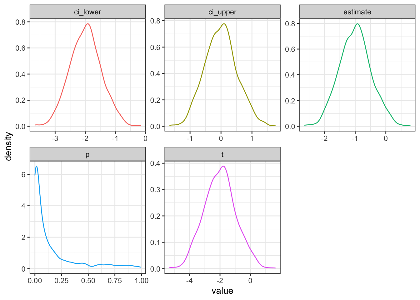
Figure 3.1: Distribution of results from simulated independent samples data
You can calculate power as the proportion of simulations on which the p-value was less than your alpha.
Your power for the parameters above is 0.496.
3.2 Paired samples
Now let’s try a paired-samples design where the variables are from a normal distribution. Each subject produces two scores (in conditions A and B). What we need to know about these two scores is:
- How many subjects?
- What are the score means?
- What are the score variances (or SDs)?
- What is the correlation between the scores?
3.2.1 Parameters
In a paired-samples design, the larger the correlation between your variables, the higher the power of your test. Imagine a case where A and B are perfectly correlated, such that B is always equal to A plus 1. This means there is no variance at all in the difference scores (they are all exactly 1) and you have perfect power to detect any effect. If A and B are not correlated at all, the power of a paired-samples test is identical to an independent-samples test with the same parameters.
3.2.3 Check your data
Now check your data; faux has a function get_params() that gives you the correlation table, means, and SDs for each numeric column in a data table.
| n | var | A | B | mean | sd |
|---|---|---|---|---|---|
| 100 | A | 1.00 | 0.54 | 9.47 | 2.68 |
| 100 | B | 0.54 | 1.00 | 10.65 | 2.57 |
3.2.4 Analysis
Finally, you can analyse your simulated data.
##
## Paired t-test
##
## data: dat$A and dat$B
## t = -4.6924, df = 99, p-value = 8.674e-06
## alternative hypothesis: true difference in means is not equal to 0
## 95 percent confidence interval:
## -1.6762660 -0.6799322
## sample estimates:
## mean of the differences
## -1.1780993.2.5 Function
The function is set up the same way as before. Set the arguments to the relevant parameters, construct the data table, run the t-test, and return the values you care about.
paired_sim <- function(sub_n, A_mean, B_mean, A_sd, B_sd, AB_r) {
dat <- faux::rnorm_multi(
    n = sub_n,
    vars = 2,
    r = AB_r,
    mu = c(A_mean, B_mean),
    sd = c(A_sd, B_sd),
    varnames = c("A", "B")
  )
t <- t.test(dat$A, dat$B, paired = TRUE)
# return just the values you care about
list(
t = t$statistic[[1]],
ci_lower = t$conf.int[[1]],
ci_upper = t$conf.int[[2]],
p = t$p.value[[1]],
estimate = t$estimate[[1]]
)
}Run 1000 simulations and graph the results.
mysim_p %>%
  gather(stat, value, t:estimate) %>%
  ggplot() +
  geom_density(aes(value, color = stat), show.legend = FALSE) +
  facet_wrap(~stat, scales = "free")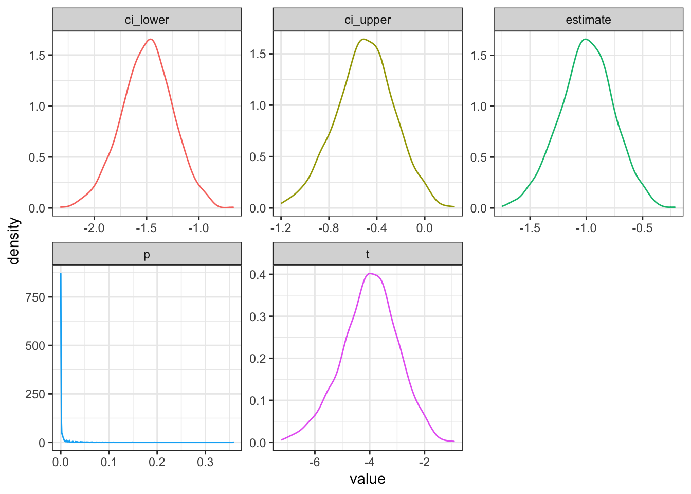
Figure 3.2: Distribution of results from simulated paired samples data
Your power for the parameters above is 0.984.
3.3 Intercept model
Now I’m going to show you a different way to simulate the same design. This might seem excessively complicated, but you will need this pattern when you start simulating data for mixed effects models.
3.3.1 Parameters
Remember, we used the following parameters to set up our simulation above:
From these, we can calculate the grand intercept (the overall mean regardless of condition), and the effect of condition (the mean of B minus A).
We also need to think about variance a little differently. First, calculate the pooled variance as the mean of the variances for A and B (remember, variance is SD squared).
If the SDs for A and B are very different, this suggests a more complicated data generation model. For this tutorial we’ll assume the score variance is similar for conditions A and B.
The variance of the subject intercepts is r times this pooled variance and the error variance is what is left over. We take the square root (sqrt()) to set the subject intercept and error SDs for simulation later.
You can think about the subject intercept variance as how much subjects vary in the score in general, regardless of condition. If they vary a lot, in comparison to the random “error” variation, then scores in the two conditions will be highly correlated. If they don’t vary much (or random variation from trial to trial is quite large), then scores won’t be well correlated.
3.3.2 Subject intercepts
Now we use these variables to create a data table for our subjects. Each subject gets an ID and a random intercept (sub_i). The intercept is simulated from a random normal distribution with a mean of 0 and an SD of sub_sd. This represents how much higher or lower than the average score each subject tends to be (regardless of condition).
3.3.3 Observations
Next, set up a table where each row represents one observation. We’ll use one of my favourite functions for simulation: crossing(). This creates every possible combination of the listed factors (it works the same as expand.grid(), but the results are in a more intuitive order). Here, we’re using it to create a row for each subject in each condition, since this is a fully within-subjects design.
3.3.4 Calculate the score
Next, we join the subject table so each row has the information about the subject’s random intercept and then calculate the score. I’ve done it in a few steps below for clarity. The score is just the sum of:
- the overall mean (
grand_i) - the subject-specific intercept (
sub_i) - the effect (
effect): the numeric code for condition (condition.e) multiplied by the effect of condition (AB_effect) - the error term (simulated from a normal distribution with mean of 0 and SD of
error_sd)
dat <- obs %>%
left_join(sub, by = "sub_id") %>%
mutate(
condition.e = recode(condition, "A" = -0.5, "B" = 0.5),
effect = AB_effect * condition.e,
error = rnorm(nrow(.), 0, error_sd),
score = grand_i + sub_i + effect + error
)
The variable condition.e “effect codes” condition, which we will use later in a mixed effect model. You can learn more about coding schemes here.
You can use the following code to put the data table into a more familiar “wide” format.
Then you can use the get_params function to check this looks correct (remove the subject ID to leave it out of the table, since it’s numeric).
| n | var | A | B | mean | sd |
|---|---|---|---|---|---|
| 100 | A | 1.00 | 0.42 | 10.46 | 2.53 |
| 100 | B | 0.42 | 1.00 | 10.78 | 2.68 |
3.3.5 Analyses
You can analyse the data with a paired-samples t-test from the wide format:
##
## Paired t-test
##
## data: dat_wide$A and dat_wide$B
## t = -1.1408, df = 99, p-value = 0.2567
## alternative hypothesis: true difference in means is not equal to 0
## 95 percent confidence interval:
## -0.8812060 0.2378312
## sample estimates:
## mean of the differences
## -0.3216874Or in the long format:
##
## Paired t-test
##
## data: score by condition
## t = -1.1408, df = 99, p-value = 0.2567
## alternative hypothesis: true difference in means is not equal to 0
## 95 percent confidence interval:
## -0.8812060 0.2378312
## sample estimates:
## mean of the differences
## -0.3216874You can analyse the data with ANOVA using the aov_4() function from afex. (Notice how the F-value is the square of the t-value above.)
## Anova Table (Type 3 tests)
##
## Response: score
## Effect df MSE F ges p.value
## 1 condition.e 1, 99 3.98 1.30 .004 .257
## ---
## Signif. codes: 0 '***' 0.001 '**' 0.01 '*' 0.05 '+' 0.1 ' ' 1You can even analyse the data with a mixed effects model using the lmer function (the afex version gives you p-values, but the lme4 version does not).
lmem <- afex::lmer(score ~ condition.e + (1 | sub_id), data = dat)
broom.mixed::tidy(lmem, effects = "fixed")%>%
# nicer formatting with p-values
mutate_if(~max(.) < .001, ~as.character(signif(., 3))) %>%
kable(digits = 3)| effect | term | estimate | std.error | statistic | df | p.value |
|---|---|---|---|---|---|---|
| fixed | (Intercept) | 10.621 | 0.219 | 48.454 | 99 | 0.000 |
| fixed | condition.e | 0.322 | 0.282 | 1.141 | 99 | 0.257 |
3.4 Functions
We can put everything together into a function where you specify the subject number, means, SDs and correlation, it translates this into the intercept specification, and returns a data table.
sim_paired_data <- function(sub_n = 100,
A_mean, B_mean,
A_sd, B_sd, AB_r) {
grand_i   <- (A_mean + B_mean)/2
AB_effect <- B_mean - A_mean
pooled_var <- (A_sd^2 + B_sd^2)/2
sub_sd   <- sqrt(pooled_var * AB_r)
error_sd <- sqrt(pooled_var * (1-AB_r))
sub <- tibble(
  sub_id = 1:sub_n,
  sub_i = rnorm(sub_n, 0, sub_sd)
)
crossing(
sub_id = 1:sub_n,
condition = c("A", "B")
) %>%
left_join(sub, by = "sub_id") %>%
mutate(
condition.e = recode(condition, "A" = -0.5, "B" = +0.5),
effect = AB_effect * condition.e,
error = rnorm(nrow(.), 0, error_sd),
score = grand_i + sub_i + effect + error
) %>%
select(sub_id, condition, score) %>%
spread(condition, score)
}| n | var | A | B | mean | sd |
|---|---|---|---|---|---|
| 100 | A | 1.00 | 0.44 | 10.12 | 2.24 |
| 100 | B | 0.44 | 1.00 | 12.07 | 2.17 |
Set the sub_n to a very high number to see that the means, SDs and correlations are what you specified.
| n | var | A | B | mean | sd |
|---|---|---|---|---|---|
| 10000 | A | 1.00 | 0.24 | 0.01 | 1.01 |
| 10000 | B | 0.24 | 1.00 | 0.49 | 1.00 |
It might be more useful to create functions to translate back and forth from the distribution specification to the intercept specification.
3.4.1 Distribution to intercept specification
dist2int <- function(mu = 0, sd = 1, r = 0) {
  A_mean <- mu[1]
  # set B_mean to A_mean if mu has length 1
  B_mean <- ifelse(is.na(mu[2]), mu[1], mu[2])
  A_sd <- sd[1]
  # set B_sd to A_sd if sd has length 1
  B_sd <- ifelse(is.na(sd[2]), sd[1], sd[2])
  AB_r <- r
  pooled_var <- (A_sd^2 + B_sd^2)/2

  list(
    grand_i = (A_mean + B_mean)/2,
    AB_effect = B_mean - A_mean,
    sub_sd = sqrt(pooled_var * AB_r),
    error_sd = sqrt(pooled_var * (1-AB_r))
  )
}| grand_i | 0 |
| AB_effect | 0 |
| sub_sd | 0 |
| error_sd | 1 |
| grand_i | 102.50 |
| AB_effect | 5.00 |
| sub_sd | 7.08 |
| error_sd | 7.08 |
3.4.2 Intercept to distribution specification
int2dist <- function(grand_i = 0,
                     AB_effect = 0,
                     sub_sd = 0,
                     error_sd = 1) {
  pooled_var <- sub_sd^2 + error_sd^2

  list(
    A_mean = grand_i - 0.5 * AB_effect,
    B_mean = grand_i + 0.5 * AB_effect,
    A_sd = sqrt(pooled_var),
    B_sd = sqrt(pooled_var),
    AB_r = sub_sd^2 / pooled_var
  )
}| A_mean | 0 |
| B_mean | 0 |
| A_sd | 1 |
| B_sd | 1 |
| AB_r | 0 |
| A_mean | 100.000 |
| B_mean | 105.000 |
| A_sd | 10.013 |
| B_sd | 10.013 |
| AB_r | 0.500 |
We can then use either specification to generate data with either technique.