Intro to Faux

In this tutorial, we’ll learn how to simulate data for factorial designs using {faux}. There are more extensive examples at https://debruine.github.io/faux/.

Setup

We’ll be using 4 packages in this tutorial.

library(tidyverse) # for data wrangling
library(faux)      # for simulation
library(broom)     # for tidy analysis results
library(afex)      # for ANOVA

set.seed(8675309) # Jenny, I've got your number

A seed makes randomness reproducible. Run the following code several times. Change the seed to your favourite integer. If the seed is the same, the random numbers after it will be the same, as long as the code is always executed in the same order.

set.seed(0)
rnorm(1)
## [1] 1.262954

Normal

Let’s start with a normal distribution using the base R function rnorm(), which returns n values from a normal distribution with a mean of 0 and a standard deviation of 1.

rnorm(n = 10)
##  [1] -0.326233361  1.329799263  1.272429321  0.414641434 -1.539950042
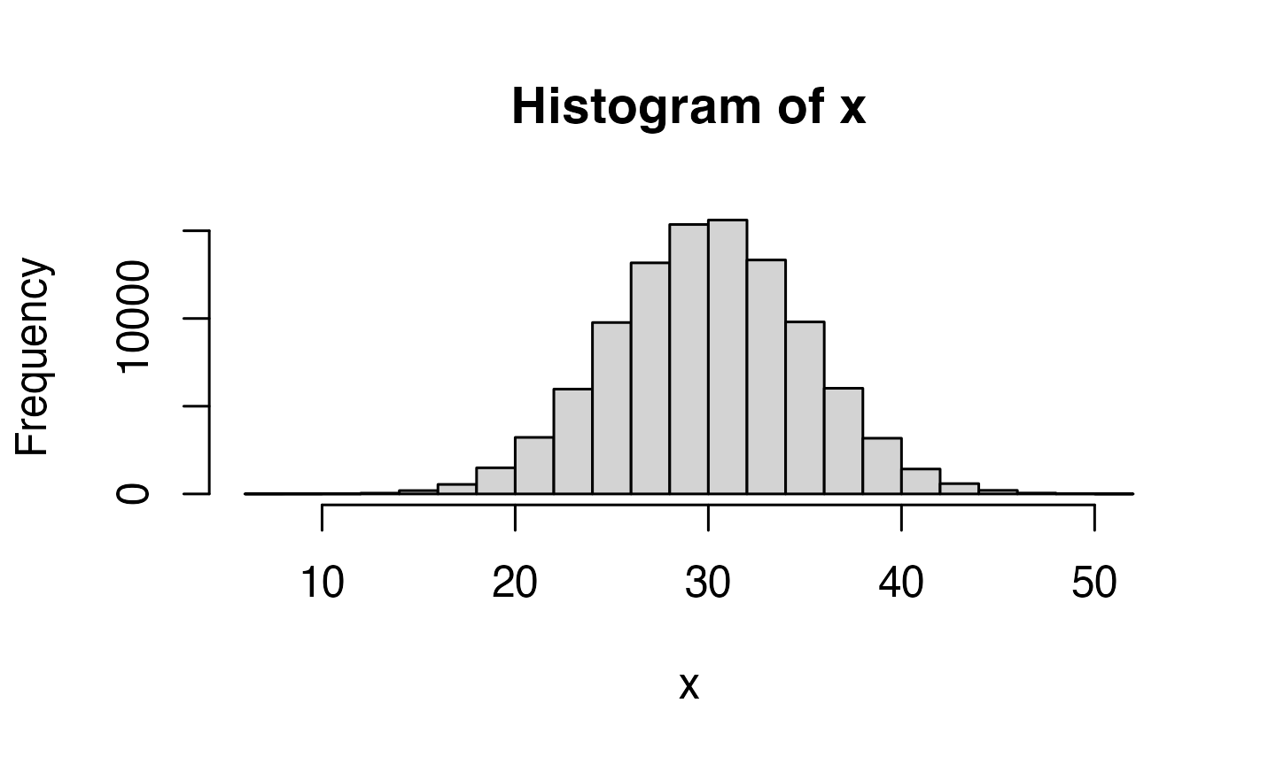
##  [6] -0.928567035 -0.294720447 -0.005767173  2.404653389  0.763593461

You can change the mean and SD. Simulate a lot of values (1e5 == 100,000), save them in a variable, and visualise them with hist().

x <- rnorm(1e5, mean = 30, sd = 5)

hist(x)

Multivariate normal

But how do you create correlated values? You can do this with MASS::mvrnorm(), but you need to construct the Sigma argument yourself from the correlation matrix and the standard deviations of the populations, and then you need to turn the resulting matrix into a data frame for many use cases. This isn’t very difficult, but can be tedious with larger numbers of variables.

n = 1e5 # this is a large number to demonstrate that the result is as expected
mu = c(A = 1, B = 2, C = 3)
sd = c(0.5, 1, 1.5)
r = c(0, .25, .5)

cor_mat <- matrix(c(1, r[1], r[2], 
                    r[1], 1, r[3],
                    r[2], r[3], 1), 
                  nrow = 3)
Sigma <- (sd %*% t(sd)) * cor_mat
vars <- MASS::mvrnorm(n, mu, Sigma) |> as.data.frame()

cor(vars) |> round(2)
##      A   B    C
## A 1.00 0.0 0.24
## B 0.00 1.0 0.50
## C 0.24 0.5 1.00

rnorm_multi

In faux, you can create sets of correlated normally distributed values using rnorm_multi().

dat3 <- rnorm_multi(
  n = 50,
  mu = c(A = 1, B = 2, C = 3),
  sd = c(0.5, 1, 1.5),
  r = c(0, .25, .5)
)

The function get_params() gives you a quick way to see the means, SDs and correlations in the simulated data set to make sure you set the parameters correctly.

get_params(dat3)
##    n var    A    B    C mean   sd
## 1 50   A 1.00 0.10 0.24 1.10 0.49
## 2 50   B 0.10 1.00 0.34 2.00 0.86
## 3 50   C 0.24 0.34 1.00 3.06 1.32

If you set empirical to TRUE, the values you set will be the sample parameters, not the population parameters. This isn’t usually what you want for a simulation, but can be useful to check you set the parameters correctly.

dat3 <- rnorm_multi(
  n = 50,
  mu = c(A = 1, B = 2, C = 3),
  sd = c(0.5, 1, 1.5),
  r = c(0, .25, .5),
  empirical = TRUE
)

get_params(dat3)
##    n var    A   B    C mean  sd
## 1 50   A 1.00 0.0 0.25    1 0.5
## 2 50   B 0.00 1.0 0.50    2 1.0
## 3 50   C 0.25 0.5 1.00    3 1.5

Setting r

You can set the r argument for correlations in a few different ways.

If all correlations have the same value, just set r equal to a single number.

# all correlations the same value
rho_same <- rnorm_multi(50, 4, r = .5, empirical = TRUE)
get_params(rho_same)
##    n var  X1  X2  X3  X4 mean sd
## 1 50  X1 1.0 0.5 0.5 0.5    0  1
## 2 50  X2 0.5 1.0 0.5 0.5    0  1
## 3 50  X3 0.5 0.5 1.0 0.5    0  1
## 4 50  X4 0.5 0.5 0.5 1.0    0  1

You can set r to a vector or matrix of the full correlation matrix. This is convenient when you’re getting the values from an existing dataset, where you can just use the output of the cor() function.

rho <- cor(iris[1:4])
round(rho, 2)
##              Sepal.Length Sepal.Width Petal.Length Petal.Width
## Sepal.Length         1.00       -0.12         0.87        0.82
## Sepal.Width         -0.12        1.00        -0.43       -0.37
## Petal.Length         0.87       -0.43         1.00        0.96
## Petal.Width          0.82       -0.37         0.96        1.00

Notice how, since we didn’t specify the names of the 4 variables anywhere else, rnorm_multi() will take them from the named correlation matrix.

rho_cormat <- rnorm_multi(50, 4, r = rho, empirical = TRUE)
get_params(rho_cormat)
##    n          var Sepal.Length Sepal.Width Petal.Length Petal.Width mean sd
## 1 50 Sepal.Length         1.00       -0.12         0.87        0.82    0  1
## 2 50  Sepal.Width        -0.12        1.00        -0.43       -0.37    0  1
## 3 50 Petal.Length         0.87       -0.43         1.00        0.96    0  1
## 4 50  Petal.Width         0.82       -0.37         0.96        1.00    0  1

Alternatively, you can just specify the values from the upper right triangle of a correlation matrix. This might be easier if you’re reading the values out of a paper.

# upper right triangle
#         X2   X3   X4
rho <- c(0.5, 0.4, 0.3, # X1
              0.2, 0.1, # X2
                   0.0) # X3

rho_urt <- rnorm_multi(50, 4, r = rho, empirical = TRUE)
get_params(rho_urt)
##    n var  X1  X2  X3  X4 mean sd
## 1 50  X1 1.0 0.5 0.4 0.3    0  1
## 2 50  X2 0.5 1.0 0.2 0.1    0  1
## 3 50  X3 0.4 0.2 1.0 0.0    0  1
## 4 50  X4 0.3 0.1 0.0 1.0    0  1

Factorial Designs

You can use rnorm_multi() to simulate data for each between-subjects cell of a factorial design and manually combine the tables, but faux has a function that better maps onto how we usually think and teach about factorial designs.

The default design is 100 observations of one variable (named y) with a mean of 0 and SD of 1. Unless you set plot = FALSE or run faux_options(plot = FALSE), this function will show you a plot of your design so you can check that it looks like you expect.

simdat1 <- sim_design()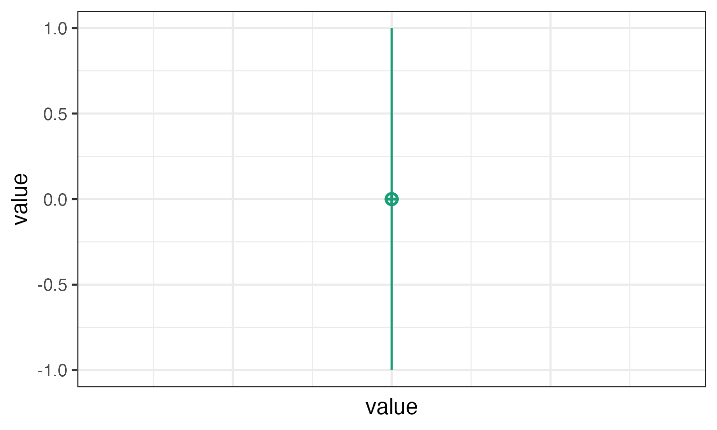

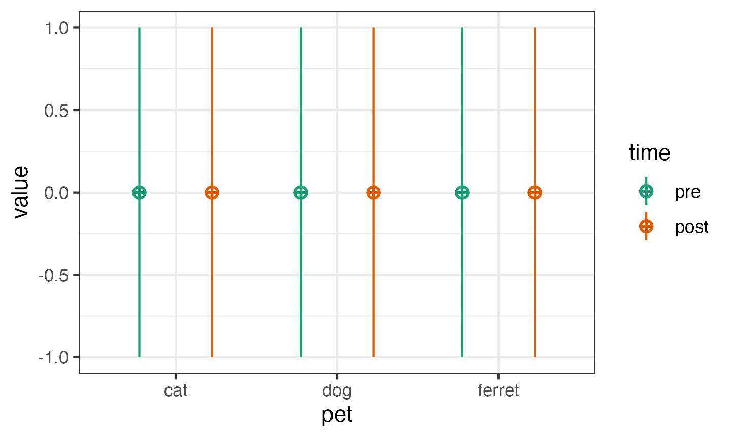
Factors

Use named lists to set the names and levels of within and between subject factors.

pettime <- sim_design(
  between = list(pet = c("cat", "dog", "ferret")),
  within = list(time = c("pre", "post"))
)

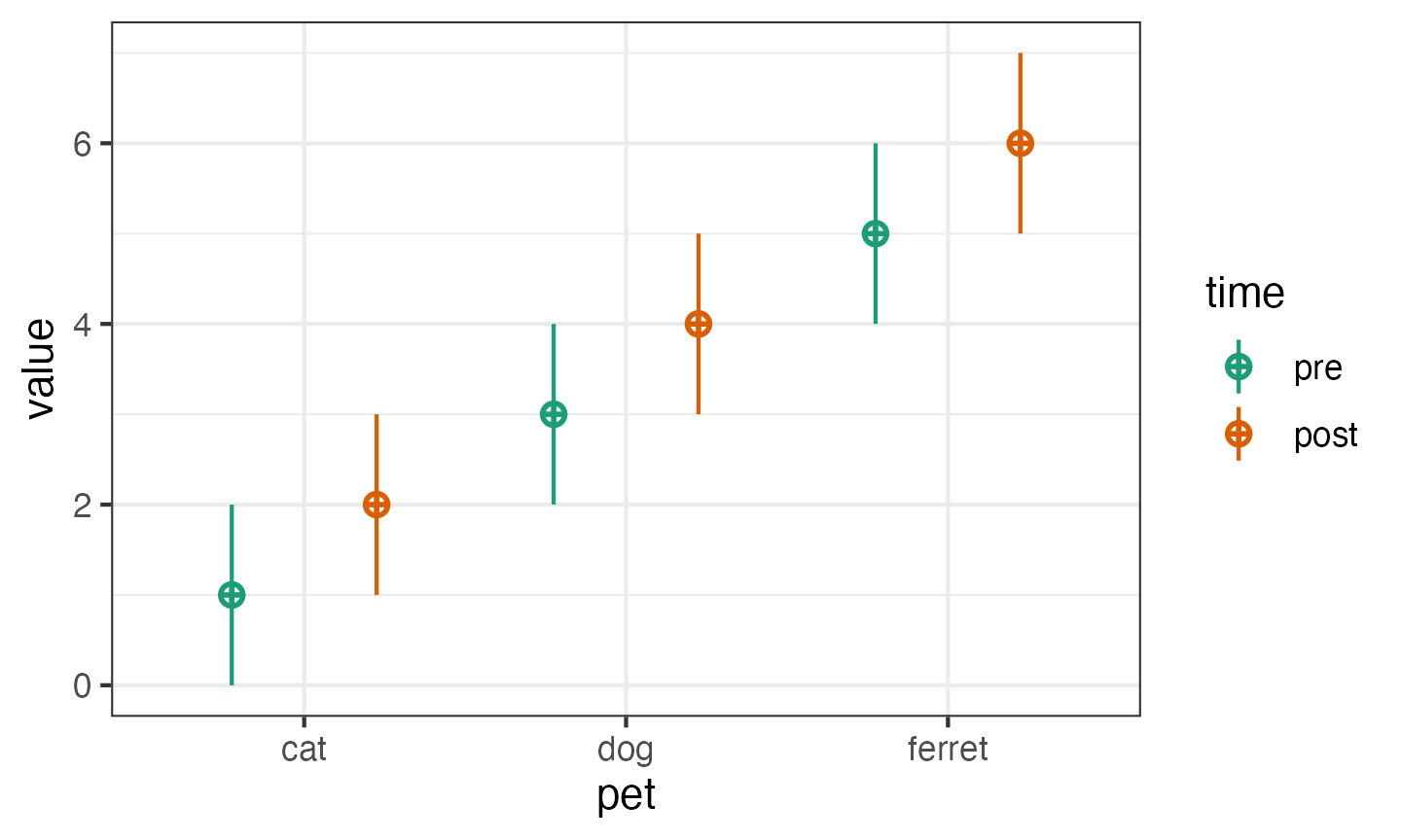
You can set mu and sd with unnamed vectors, but getting the order right can take some trial and error.

pettime <- sim_design(
  between = list(pet = c("cat", "dog", "ferret")),
  within = list(time = c("pre", "post")),
  mu = 1:6
)

You can set values with a named vector for a single type of factor. The values do not have to be in the right order if they’re named.

pettime <- sim_design(
  between = list(pet = c("cat", "dog", "ferret")),
  within = list(time = c("pre", "post")),
  mu = c(cat = 1, ferret = 5, dog = 3),
  sd = c(pre = 1, post = 2)
)

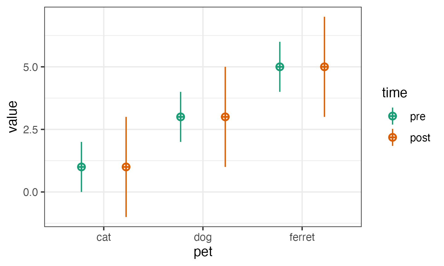
Or use a data frame for within- and between-subject factors.

pettime <- sim_design(
  between = list(pet = c("cat", "dog", "ferret")),
  within = list(time = c("pre", "post")),
  mu = data.frame(
    pre = c(1, 3, 5),
    post = c(2, 4, 6),
    row.names = c("cat", "dog", "ferret")
  )
)

If you have within-subject factors, set the correlations for each between-subject cell like this.

pettime <- sim_design(
  between = list(pet = c("cat", "dog", "ferret")),
  within = list(time = c("pre", "post")),
  r = list(cat = 0.5,
           dog = 0.25,
           ferret = 0),
  empirical = TRUE,
  plot = FALSE
)

get_params(pettime)
##      pet   n  var  pre post mean sd
## 1    cat 100  pre 1.00 0.50    0  1
## 2    cat 100 post 0.50 1.00    0  1
## 3    dog 100  pre 1.00 0.25    0  1
## 4    dog 100 post 0.25 1.00    0  1
## 5 ferret 100  pre 1.00 0.00    0  1
## 6 ferret 100 post 0.00 1.00    0  1

You can also change the name of the dv and id columns and output the data in long format. If you do this, you also need to tell get_params() what columns contain the between- and within-subject factors, the dv, and the id.

dat_long <- sim_design(
  between = list(pet = c("cat", "dog", "ferret")),
  within = list(time = c("pre", "post")),
  id = "subj_id",
  dv = "score",
  long = TRUE,
  plot = FALSE
)

get_params(dat_long, digits = 3)
##      pet   n  var    pre   post   mean    sd
## 1    cat 100  pre  1.000  0.074  0.082 0.944
## 2    cat 100 post  0.074  1.000  0.097 1.091
## 3    dog 100  pre  1.000 -0.061  0.036 1.014
## 4    dog 100 post -0.061  1.000  0.115 1.024
## 5 ferret 100  pre  1.000  0.009 -0.015 0.998
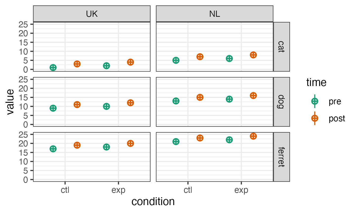
## 6 ferret 100 post  0.009  1.000 -0.115 0.887

Multiple Factors

Set more than one within-or between-subject factor like this:

dat_multi <- sim_design(
  between = list(pet = c("cat", "dog", "ferret"),
                 country = c("UK", "NL")),
  within = list(time = c("pre", "post"),
                condition = c("ctl", "exp")),
  mu = data.frame(
    cat_UK = 1:4,
    cat_NL = 5:8,
    dog_UK = 9:12,
    dog_NL = 13:16,
    ferret_UK = 17:20, 
    ferret_NL = 21:24,
    row.names = c("pre_ctl", "pre_exp", "post_ctl", "post_exp")
  )
)

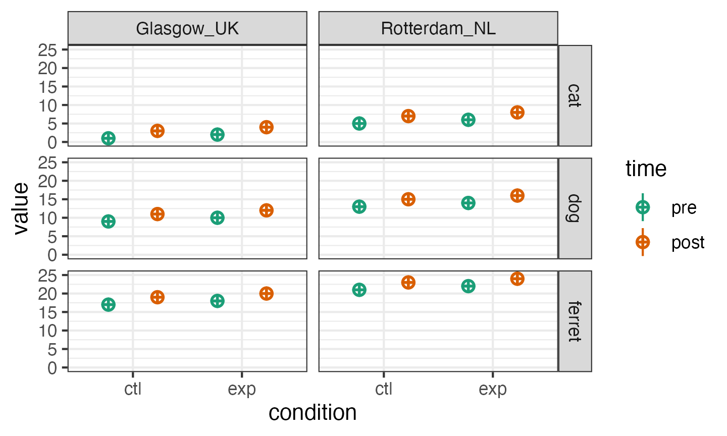
Because faux uses an underscore for the separator, you have to set the sep argument to something different if you want to use underscores in your variable names (or set the separator globally with faux_options).

# faux_options(sep = ".")

dat_multi <- sim_design(
  between = list(pet = c("cat", "dog", "ferret"),
                 country = c("Glasgow_UK", "Rotterdam_NL")),
  within = list(time = c("pre", "post"),
                condition = c("ctl", "exp")),
  mu = data.frame(
    cat.Glasgow_UK = 1:4,
    cat.Rotterdam_NL = 5:8,
    dog.Glasgow_UK = 9:12,
    dog.Rotterdam_NL = 13:16,
    ferret.Glasgow_UK = 17:20, 
    ferret.Rotterdam_NL = 21:24,
    row.names = c("pre.ctl", "pre.exp", "post.ctl", "post.exp")
  ),
  sep = "."
)

Anonymous Factors

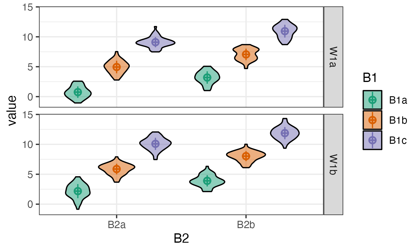
If you need to make a quick demo, you can set factors anonymously with integer vectors. For example, the following code makes 3B*2B*2W mixed design.

dat_anon <- sim_design(
  n = 50,
  between = c(3, 2),
  within = 2,
  mu = 1:12
)

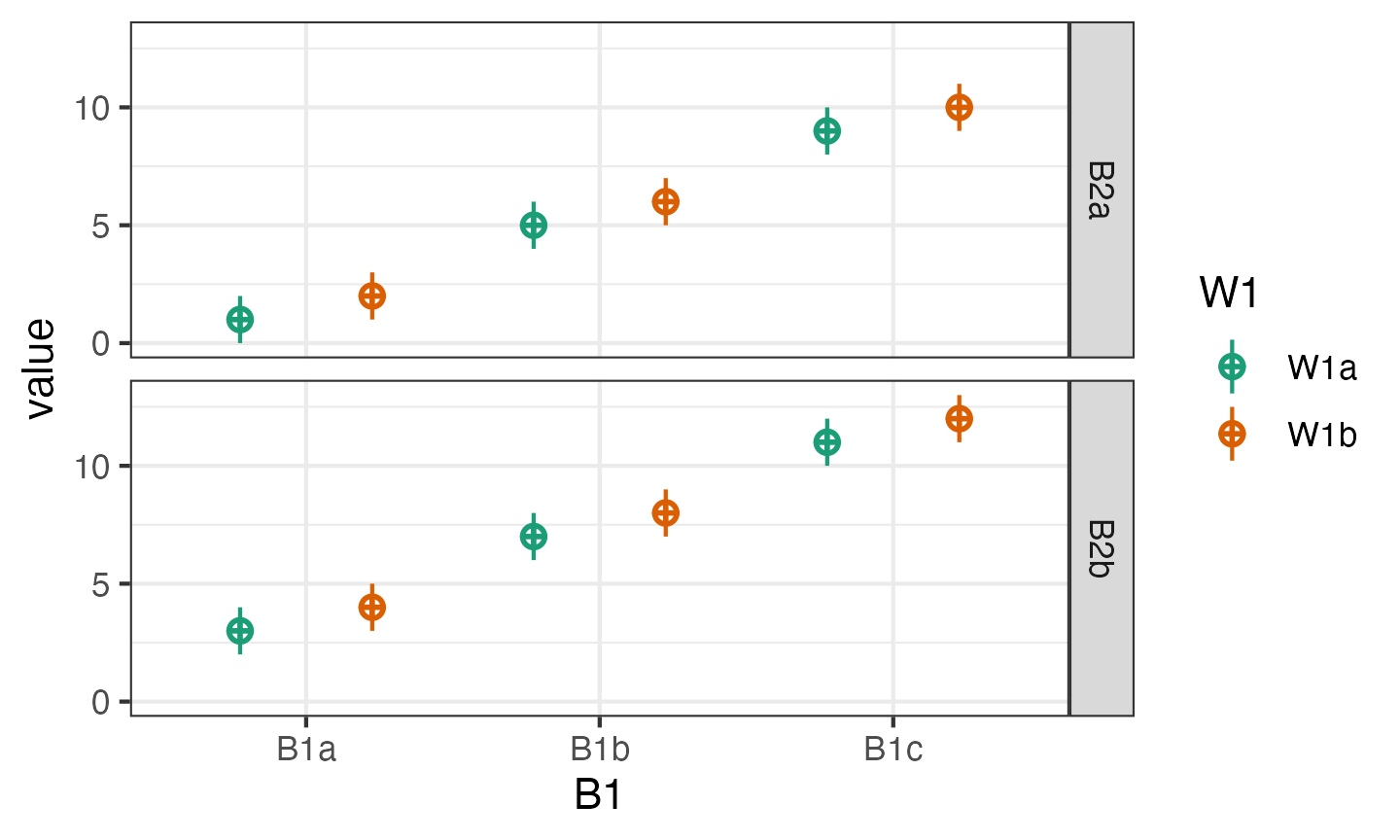
Faux has a quick plotting function for visualising data made with faux. The plot created by sim_design() shows the design, while this function shows the simulated data.

plot(dat_anon)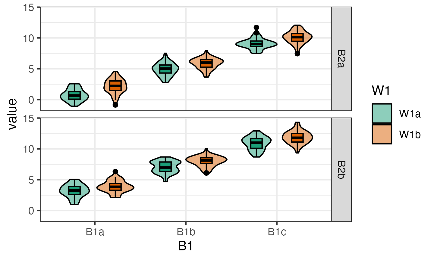

You can change the order of plotting and the types of geoms plotted. This takes a little trial and error, so this function will probably be refined in later versions.

plot(dat_anon, "B1", "B2", "W1", geoms = c("violin", "pointrangeSD"))

Replications

You often want to simulate data repeatedly to do things like calculate power. The sim_design() function has a lot of overhead for checking if a design makes sense and if the correlation matrix is possible, so you can speed up the creation of multiple datasets with the same design using the rep argument. This will give you a nested data frame with each dataset in the data column.

dat_rep <- sim_design(
  within = 2,
  n = 20,
  mu = c(0, 0.25),
  rep = 5,
  plot = FALSE
)

Analyse each replicate

You can run analyses on the nested data by wrapping your analysis code in a function then using map() to run the analysis on each data set and unnest() to expand the results into a data table.

# define function
analyse <- function(data) {
  t.test(data$W1a, data$W1b, paired = TRUE) %>% broom::tidy()
}

# get one test data set
data <- dat_rep$data[[1]]

# check function returns what you want
analyse(data)
## # A tibble: 1 × 8
##   estimate statistic p.value parameter conf.low conf.high method     alternative
##      <dbl>     <dbl>   <dbl>     <dbl>    <dbl>     <dbl> <chr>      <chr>      
## 1   -0.528     -1.96  0.0647        19    -1.09    0.0354 Paired t-… two.sided

# run the function on each data set
dat_rep |>
  mutate(analysis = map(data, analyse)) |>
  select(-data) |>
  unnest(analysis)
## # A tibble: 5 × 9
##     rep estimate statistic p.value parameter conf.low conf.high method       
##   <int>    <dbl>     <dbl>   <dbl>     <dbl>    <dbl>     <dbl> <chr>        
## 1     1  -0.528    -1.96    0.0647        19   -1.09     0.0354 Paired t-test
## 2     2  -0.532    -2.68    0.0147        19   -0.947   -0.117  Paired t-test
## 3     3   0.0199    0.0701  0.945         19   -0.576    0.616  Paired t-test
## 4     4  -0.111    -0.311   0.759         19   -0.856    0.635  Paired t-test
## 5     5  -0.856    -2.02    0.0576        19   -1.74     0.0305 Paired t-test
## # ℹ 1 more variable: alternative <chr>

ANOVA

Use the same pattern to run an ANOVA on a version of the pettime dataset.

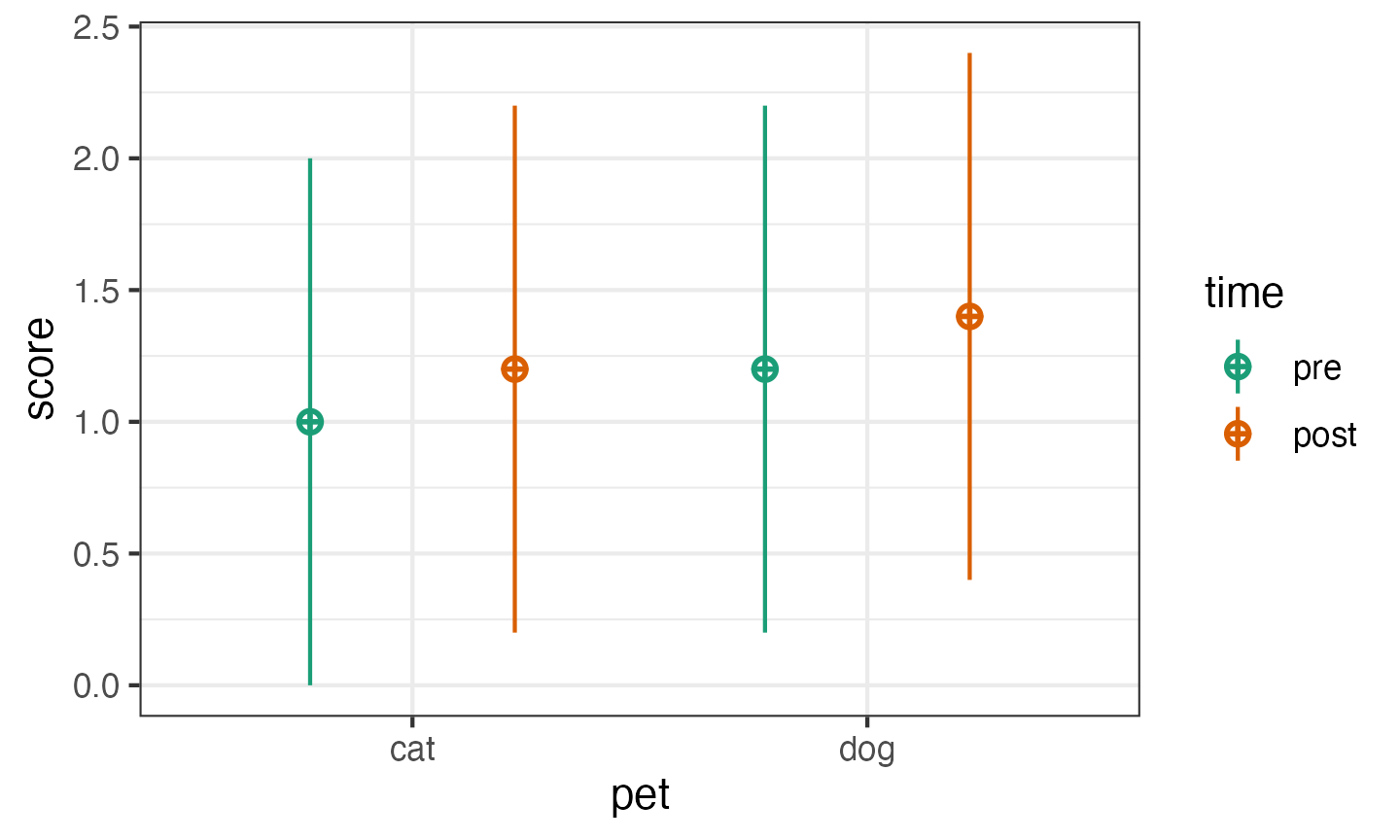
First, simulate 100 datasets in long format. These data will have small main effects of pet and time, but no interaction.

pettime100 <- sim_design(
  between = list(pet = c("cat", "dog")),
  within = list(time = c("pre", "post")),
  n = c(cat = 50, dog = 40),
  mu = data.frame(
    pre = c(1, 1.2),
    post = c(1.2, 1.4),
    row.names = c("cat", "dog")
  ),
  sd = 1,
  id = "pet_id",
  dv = "score",
  r = 0.5,
  long = TRUE,
  rep = 100
)

Then set up your analysis. We’ll use the aov_ez() function from the {afex} package because its arguments match those of sim_design(). There’s a little setup to run first to get rid of annoying messages and make this run faster by omitting calculations we won’t need.

afex::set_sum_contrasts() # avoids annoying afex message
## setting contr.sum globally: options(contrasts=c('contr.sum', 'contr.poly'))
afex_options(include_aov = FALSE) # runs faster
afex_options(es_aov = "pes") # changes effect size measure to partial eta squared

This custom function takes the data frame as input and runs our ANOVA on it. The code at the end just cleans up the resulting table a bit.

analyse <- function(data) {
  a <- afex::aov_ez(
    id = "pet_id",
    dv = "score",
    between = "pet",
    within = "time",
    data = data
  ) 
  # return anova_table for GG-corrected DF
  as_tibble(a$anova_table, rownames = "term") |>
    mutate(term = factor(term, levels = term)) |> # keeps terms in order
    rename(p.value = `Pr(>F)`) # fixes annoying p.value name
}

Test the analysis code on the first simulated data frame.

analyse( pettime100$data[[1]] )
## # A tibble: 3 × 7
##   term     `num Df` `den Df`   MSE     F     pes p.value
##   <fct>       <dbl>    <dbl> <dbl> <dbl>   <dbl>   <dbl>
## 1 pet             1       88 1.42  0.693 0.00781  0.408 
## 2 time            1       88 0.466 4.76  0.0513   0.0318
## 3 pet:time        1       88 0.466 0.166 0.00189  0.684

Use the same code we used in the first example to make a table of the results of each analysis:

pettime_sim <- pettime100 |>
  mutate(analysis = map(data, analyse)) |>
  select(-data) |>
  unnest(analysis)

## # A tibble: 6 × 8
##     rep term     `num Df` `den Df`   MSE     F   pes p.value
##   <int> <fct>       <dbl>    <dbl> <dbl> <dbl> <dbl>   <dbl>
## 1     1 pet             1       88 1.42  0.693 0.008   0.408
## 2     1 time            1       88 0.466 4.76  0.051   0.032
## 3     1 pet:time        1       88 0.466 0.166 0.002   0.684
## 4     2 pet             1       88 1.94  4.32  0.047   0.04 
## 5     2 time            1       88 0.506 1.86  0.021   0.177
## 6     2 pet:time        1       88 0.506 1.49  0.017   0.225

Then you can summarise the data to calculate things like power for each effect or mean effect size.

pettime_sim |>
  group_by(term) |>
  summarise(power = mean(p.value < 0.05),
            mean_pes = mean(pes) |> round(3),
            .groups = "drop")
## # A tibble: 3 × 3
##   term     power mean_pes
##   <fct>    <dbl>    <dbl>
## 1 pet       0.2     0.024
## 2 time      0.45    0.05 
## 3 pet:time  0.04    0.01

The power for the between-subjects effect of pet is smaller than for the within-subjects effect of time. What happens if you reduce the correlation between pre and post?

Non-normal Distributions

The newest version of faux has a new function for simulating non-normal distributions using the NORTA method (NORmal To Anything). The dist argument lists the variables with their distribution names (e.g., “norm”, “pois”, unif”, “truncnorm”, or anything that has an “rdist” function). The params argument lists the distribution function argument values for each variable (e.g., arguments to rnorm, rpois, runif, rtruncnorm).

This function simulates multivariate non-normal distributions by using simulation to work out the correlations for a multivariate normal distribution that will produce the desired correlations after the normal distributions are converted to the desired distributions. This simulation can take a while if you have several variables and should warn you if you’re requesting an impossible combination (but is still an experimental function, so let Lisa know if you have any problems).

dat_norta <- rmulti(
  n = 1000,
  dist = c(U = "unif",
           T = "truncnorm",
           L = "likert"),
  params = list(
    U = list(min = 0, max = 10),
    T = list(a = 1, b = 7, mean = 3.5, sd = 2.1),
    L = list(prob = c(`much less` = .10, 
                      `less`      = .20, 
                      `equal`     = .35, 
                      `more`      = .25, 
                      `much more` = .10))
  ),
  r = c(-0.5, 0, 0.5)
)

The “likert” type is a set of distribution functions provided by faux to make creating Likert scale variables easier (see ?rlikert). You may need to convert Likert-scale variables to numbers before analysis or calculating descriptives.

# convert likert-scale variable to integer
dat_norta$L <- as.integer(dat_norta$L)

get_params(dat_norta)
##      n var     U     T     L mean   sd
## 1 1000   U  1.00 -0.46 -0.01 4.98 2.88
## 2 1000   T -0.46  1.00  0.52 3.67 1.46
## 3 1000   L -0.01  0.52  1.00 3.02 1.11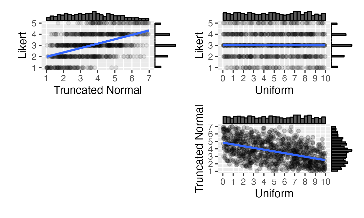

Exercises

Multivariate normal

Sample 40 values of three variables named J, K and L from a population with means of 10, 20 and 30, and SDs of 5. J and K are correlated 0.5, J and L are correlated 0.25, and K and L are not correlated.

From existing data

Using the data from the built-in dataset attitude, simulate a new set of 20 observations drawn from a population with the same means, SDs and correlations for each column as the original data.

2b

Create a dataset with a between-subject factor of “pet” having two levels, “cat”, and “dog”. The DV is “happiness” score. There are 20 cat-owners with a mean happiness score of 10 (SD = 3) and there are 30 dog-owners with a mean happiness score of 11 (SD = 3).

3w

Create a dataset of 20 observations with 1 within-subject variable (“condition”) having 3 levels (“A”, “B”, “C”) with means of 10, 20 and 30 and SD of 5. The correlations between each level have r = 0.4. The dataset should look like this:

id	condition	score
S01	A	9.17
…	…	…
S20	A	11.57
S01	B	18.44
…	…	…
S20	B	20.04
S01	C	35.11
…	…	…
S20	C	29.16

2w*2w

Create a dataset with 50 observations of 2 within-subject variables (“W1” and “W2”) each having 2 levels. The mean for all cells is 10 and the SD is 2. The dataset should have 20 subjects. The correlations look like this:

	W1a_W2a	W1a_W2b	W1b_W2a	W1b_W2b
W1a_W2a	1.0	0.5	0.5	0.2
W1a_W2b	0.5	1.0	0.2	0.5
W1b_W2a	0.5	0.2	1.0	0.5
W1b_W2b	0.2	0.5	0.5	1.0

2w*3b

Create a dataset with a between-subject factor of “pet” having 3 levels (“cat”, “dog”, and “ferret”) and a within-subject factor of “time” having 2 levels (“pre” and “post”). The N in each group should be 10. Means are:

cats: pre = 10, post = 12
dogs: pre = 14, post = 16
ferrets: pre = 18, post = 20

SDs are all 5 and within-cell correlations are all 0.25.

Replications

Create 5 datasets with a 2b*2b design, 30 participants in each cell. Each cell’s mean should be 0, except B1a:B2a, which should be 0.5. The SD should be 1. Make the resulting data in long format.

Power

Simulate 100 datasets like the one above and use lm() or afex::aov_ez() to look at the interaction between A and B. What is the power of this design?

Lisa DeBruine

Setup

Normal

Multivariate normal

rnorm_multi

Setting r

Factorial Designs

Factors

Multiple Factors

Anonymous Factors

Replications

Analyse each replicate

ANOVA

Non-normal Distributions

Exercises

Multivariate normal

From existing data

2b

3w

2w*2w

2w*3b

Replications

Power