Fixed Effects

Lisa DeBruine

library(tidyverse)
library(faux)
library(afex) # for anova and lmer
library(broom)
library(broom.mixed) # to make tidy tables of lmer output

theme_set(theme_minimal(base_size = 14))

Simulation functions

The functions below are commonly used when you’re setting up a simulated dataset.

Repeating

The function rep() lets you repeat the first argument a number of times.

Use rep() to create a vector of alternating "A" and "B" values of length 24.

rep(c("A", "B"), times = 12)
##  [1] "A" "B" "A" "B" "A" "B" "A" "B" "A" "B" "A" "B" "A" "B" "A" "B" "A" "B" "A"
## [20] "B" "A" "B" "A" "B"

If the second argument is a vector that is the same length as the first argument, each element in the first vector is repeated that many times. Use rep() to create a vector of 11 "A" values followed by 3 "B" values.

rep(c("A", "B"), c(11, 3))
##  [1] "A" "A" "A" "A" "A" "A" "A" "A" "A" "A" "A" "B" "B" "B"

You can repeat each element of the vector a specified number of times using the each argument, Use rep() to create a vector of 12 "A" values followed by 12 "B" values.

rep(c("A", "B"), each = 12)
##  [1] "A" "A" "A" "A" "A" "A" "A" "A" "A" "A" "A" "A" "B" "B" "B" "B" "B" "B" "B"
## [20] "B" "B" "B" "B" "B"

What do you think will happen if you set times to 3 and each to 2?

rep(c("A", "B"), times = 3, each = 2)
##  [1] "A" "A" "B" "B" "A" "A" "B" "B" "A" "A" "B" "B"

Sequences

The function seq() is useful for generating a sequence of numbers with some pattern.

Use seq() to create a vector of the integers 0 to 10.

seq(0, 10)
##  [1]  0  1  2  3  4  5  6  7  8  9 10

You can set the by argument to count by numbers other than 1 (the default). Use seq() to create a vector of the numbers 0 to 100 by 10s.

seq(0, 100, by = 10)
##  [1]   0  10  20  30  40  50  60  70  80  90 100

The argument length.out is useful if you know how many steps you want to divide something into. Use seq() to create a vector that starts with 0, ends with 100, and has 12 equally spaced steps (hint: how many numbers would be in a vector with 2 steps?).

seq(0, 100, length.out = 13)
##  [1]   0.000000   8.333333  16.666667  25.000000  33.333333  41.666667
##  [7]  50.000000  58.333333  66.666667  75.000000  83.333333  91.666667
## [13] 100.000000

Uniform Distribution

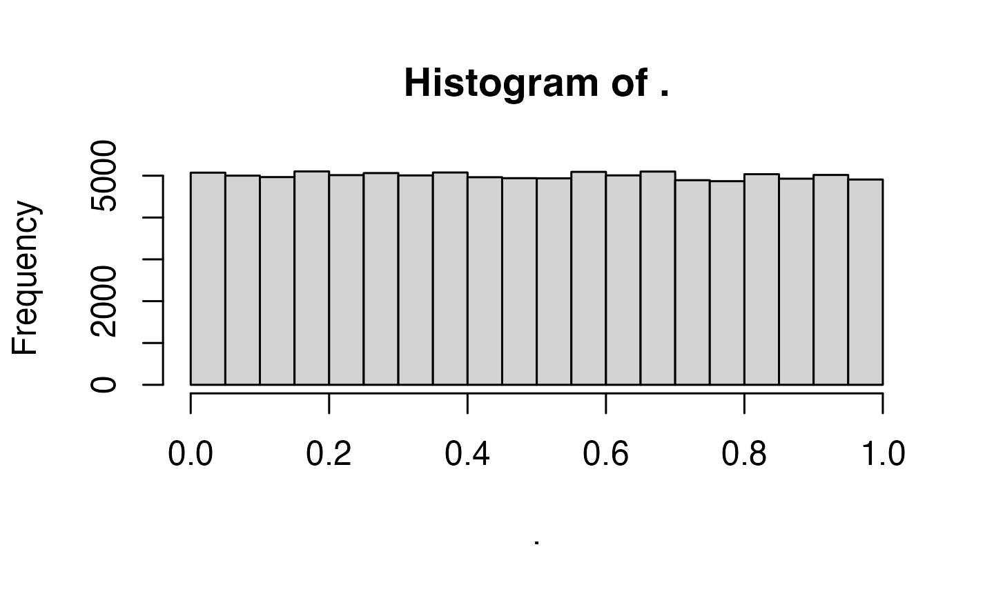
The uniform distribution is the simplest distribution. All numbers in the range have an equal probability of being sampled. Use runif() to sample from a continuous uniform distribution.

runif(n = 10, min = 0, max = 1)
##  [1] 0.1594836 0.4781883 0.7647987 0.7696877 0.2685485 0.6730459 0.9787908
##  [8] 0.8463270 0.8566562 0.4451601

Pipe the result to hist() to make a quick histogram of your simulated data.

runif(100000, min = 0, max = 1) %>% hist()

Discrete Distribution

You can use sample() to simulate events like rolling dice or choosing from a deck of cards. The code below simulates rolling a 6-sided die 10000 times. We set replace to TRUE so that each event is independent. See what happens if you set replace to FALSE.

rolls <- sample(1:6, 10000, replace = TRUE)

# plot the results
as.factor(rolls) %>% plot()

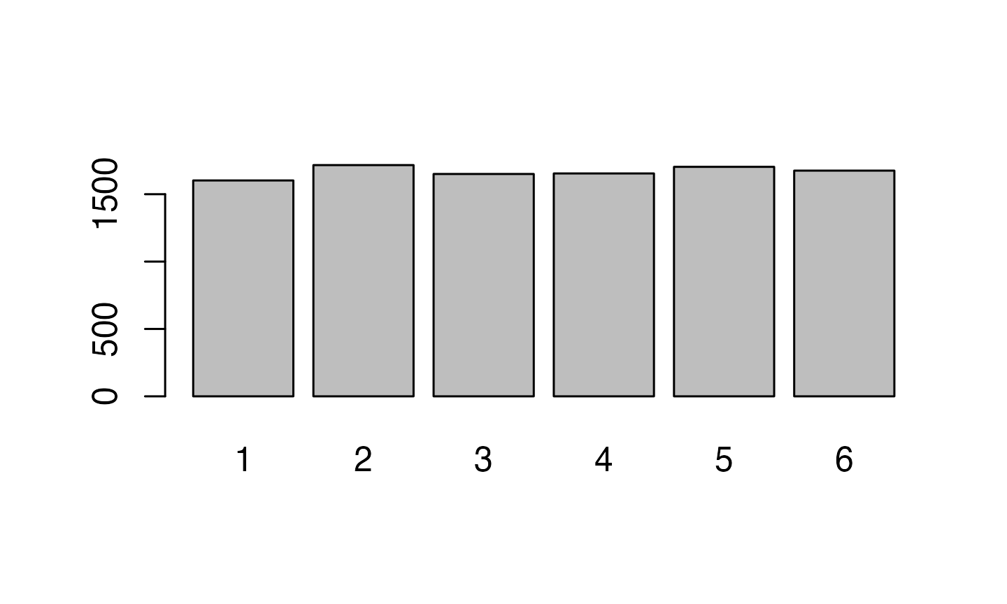
Distribution of dice rolls.

You can also use sample to sample from a list of named outcomes.

pet_types <- c("cat", "dog", "ferret", "bird", "fish")
sample(pet_types, 10, replace = TRUE)
##  [1] "dog"    "fish"   "cat"    "fish"   "bird"   "bird"   "fish"   "ferret"
##  [9] "ferret" "bird"

Ferrets, while the best pet, are a much less common pet than cats and dogs, so our sample isn’t very realistic. You can set the probabilities of each item in the list with the prob argument.

pet_types <- c("cat", "dog", "ferret", "bird", "fish")
pet_prob <- c(0.3, 0.4, 0.1, 0.1, 0.1)
pet_data <- sample(pet_types, 100, replace = TRUE, prob = pet_prob) 

as.factor(pet_data) %>% plot()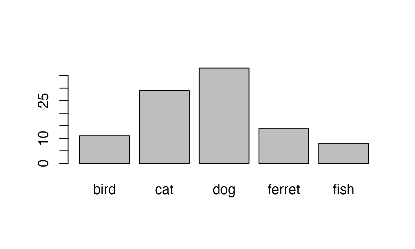

Binomial Distribution

The rbinom function will generate a random binomial distribution.

• n = number of observations
• size = number of trials
• prob = probability of success on each trial

Coin flips are a typical example of a binomial distribution, where we can assign heads to 1 and tails to 0.

# 20 individual coin flips of a fair coin
rbinom(20, 1, 0.5)
##  [1] 0 1 1 0 0 0 1 0 1 0 0 0 0 1 0 1 0 0 0 1

# 20 individual coin flips of a baised (0.75) coin
rbinom(20, 1, 0.75)
##  [1] 1 1 1 0 1 1 1 1 1 1 1 1 1 0 1 1 1 1 0 1

You can generate the total number of heads in 1 set of 20 coin flips by setting size to 20 and n to 1.

# 1 set of 20 fair coin flips
rbinom(1, 20, 0.75)
## [1] 13

You can generate more sets of 20 coin flips by increasing the n.

# 10 sets of 20 fair coin flips
rbinom(10, 20, 0.5)
##  [1] 12  7 10 11 11  8 11  7 12  8

Normal Distribution

We can simulate a normal distribution of size n if we know the mean and standard deviation (sd).

# 10 samples from a normal distribution with a mean of 0 and SD of 1
rnorm(10, 0, 1)
##  [1] -0.3230057  0.7213149  0.4248971  1.4033239 -0.6881243 -0.2737261
##  [7] -0.1539815 -0.3908546 -0.3301087  1.7890306

A density plot is usually the best way to visualise this type of data.

# 100 samples from a normal distribution with a mean of 10 and SD of 2
dv <- rnorm(100, 10, 2)

# use sample to get a random colour
fill_colour <- sample(colours(), 1)

ggplot() +
  geom_density(aes(dv), fill = fill_colour) +
  scale_x_continuous(
    limits = c(0,20), 
    breaks = seq(0,20)
  )

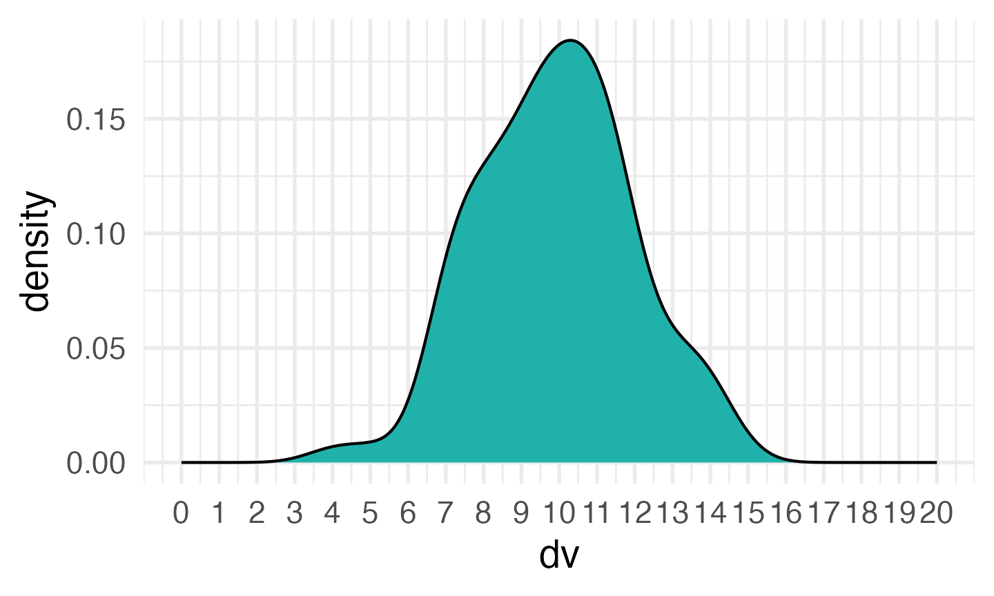
Run the simulation above several times, noting how the density plot changes. Try changing the values of n, mean, and sd.

Independent samples

Now we’re ready to start simulating some data. Let’s start with a simple independent-samples design where the variables are from a normal distribution. Each subject produces one score (in condition A or B). What we need to know about these scores is:

• How many subjects are in each condition?
• What are the score means?
• What are the score variances (or SDs)?

Parameters

First, set parameters for these values. This way, you can use these variables wherever you need them in the rest of the code and you can easily change them.

A_sub_n <- 50
B_sub_n <- 50
A_mean  <- 10
B_mean  <- 11
A_sd    <- 2.5
B_sd    <- 2.5

Scores

We can the generate the scores using the rnorm() function.

A_scores <- rnorm(A_sub_n, A_mean, A_sd)
B_scores <- rnorm(B_sub_n, B_mean, B_sd)

You can stop here and just analyse your simulated data with t.test(A_scores, B_scores), but usually you want to get your simulated data into a data table that looks like what you might eventually import from a CSV file with your actual experimental data.

dat <- tibble(
  sub_condition = rep( c("A", "B"), c(A_sub_n, B_sub_n) ),
  score = c(A_scores, B_scores)
)

If you’re simulating data for a script where you will eventually import data from a csv file, you can save these data to a csv file and then re-read them in, so when you get your real data, all you need to do is comment out the simulation steps.

# make a data directory if there isn't one already
if (!dir.exists("data")) dir.create("data")

# save your simulated data
write_csv(dat, "data/sim-data-ind-samples.csv")

# start your analysis here
dat <- read_csv("data/sim-data-ind-samples.csv")
## Rows: 100 Columns: 2
## ── Column specification ────────────────────────────────────────────────────────
## Delimiter: ","
## chr (1): sub_condition
## dbl (1): score
## 
## ℹ Use `spec()` to retrieve the full column specification for this data.
## ℹ Specify the column types or set `show_col_types = FALSE` to quiet this message.

Check your data

Always examine your simulated data after you generate it to make sure it looks like you want.

dat %>%
  group_by(sub_condition) %>%
  summarise(n = n() ,
            mean = mean(score),
            sd = sd(score),
            .groups = "drop")
## # A tibble: 2 × 4
##   sub_condition     n  mean    sd
##   <chr>         <int> <dbl> <dbl>
## 1 A                50  10.3  2.54
## 2 B                50  10.8  2.38

Analysis

t.test(score~sub_condition, dat)
## 
##  Welch Two Sample t-test
## 
## data:  score by sub_condition
## t = -0.99215, df = 97.577, p-value = 0.3236
## alternative hypothesis: true difference in means between group A and group B is not equal to 0
## 95 percent confidence interval:
##  -1.4645314  0.4882661
## sample estimates:
## mean in group A mean in group B 
##        10.31599        10.80412

Function

You can wrap all this in a function so you can run it many times to do a power calculation. Put all your parameters as arguments to the function.

ind_sim <- function(A_sub_n, B_sub_n, 
                    A_mean, B_mean, 
                    A_sd, B_sd) {
  # simulate data for groups A and B
  A_scores <- rnorm(A_sub_n, A_mean, A_sd)
  B_scores <- rnorm(B_sub_n, B_mean, B_sd)
  
  # put the data into a table
  dat <- tibble(
    sub_condition = rep( c("A", "B"), c(A_sub_n, B_sub_n) ),
    score = c(A_scores, B_scores)
  )
  
  # analyse the data
  t <- t.test(score~sub_condition, dat)
  
  # return a list of the values you care about
  # the double brackets ([[]]) get rid of the name of named numbers
  list(
    t = t$statistic[[1]],
    ci_lower = t$conf.int[[1]],
    ci_upper = t$conf.int[[2]],
    p = t$p.value[[1]],
    estimate = t$estimate[[1]] - t$estimate[[2]]
  )
}

Now run your new function with the values you used above.

# str() prints the resulting list in a shorter format
ind_sim(50, 50, 10, 11, 2.5, 2.5) %>% str()
## List of 5
##  $ t       : num -2.18
##  $ ci_lower: num -2.11
##  $ ci_upper: num -0.101
##  $ p       : num 0.0314
##  $ estimate: num -1.1

Now you can use this function to run many simulations. The function map_df from the purrr package (loaded with tidyverse) is one of many ways to run a function many times and organise the results into a table.

mysim <- map_df(1:1000, ~ind_sim(50, 50, 10, 11, 2.5, 2.5))

Now you can graph the data from your simulations.

# set boundary = 0 when plotting p-values
ggplot(mysim, aes(p)) +
  geom_histogram(binwidth = 0.05, boundary = 0,
                 fill = "white", colour = "black")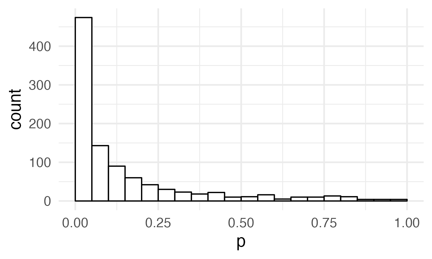

mysim %>%
  gather(stat, value, t:estimate) %>%
  ggplot() + 
  geom_density(aes(value, color = stat), show.legend = FALSE) +
  facet_wrap(~stat, scales = "free")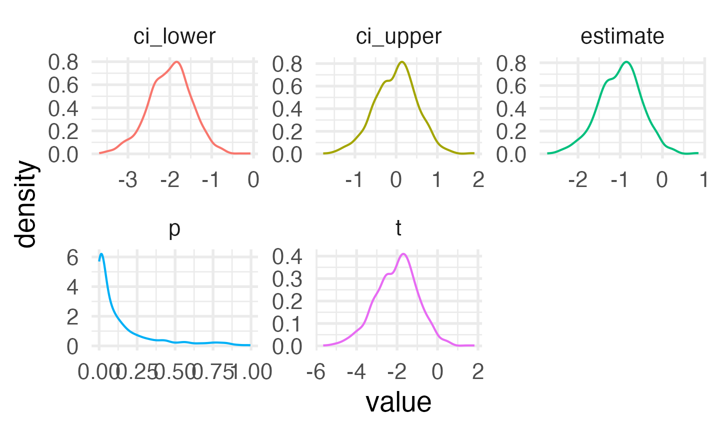

Distribution of results from simulated independent samples data

You can calculate power as the proportion of simulations on which the p-value was less than your alpha.

alpha <- 0.05
power <- mean(mysim$p < alpha)
power
## [1] 0.474

Paired samples

Now let’s try a paired-samples design where the variables are from a normal distribution. Each subject produces two scores (in conditions A and B). What we need to know about these two scores is:

• How many subjects?
• What are the score means?
• What are the score variances (or SDs)?
• What is the correlation between the scores?

Parameters

sub_n <- 100
A_mean <- 10
B_mean <- 11
A_sd <- 2.5
B_sd <- 2.5
AB_r <- 0.5

Correlated Scores

You can then use rnorm_multi() to generate a data table with simulated values for correlated scores:

dat <- faux::rnorm_multi(
    n = sub_n, 
    vars = 2, 
    r = AB_r, 
    mu = c(A_mean, B_mean), 
    sd = c(A_sd, B_sd), 
    varnames = c("A", "B")
  )

You can also do this using the MASS::mvrnorm function, but faux::rnorm_multi is easier when you have more variables to simulate.

# make the correlation matrix
cormat <- matrix(c(   1, AB_r,
                   AB_r,    1), 
             nrow = 2, byrow = TRUE)

# make a corresponding matrix of the variance 
# (multiply the SDs for each cell)
varmat <- matrix(c(A_sd * A_sd, A_sd * B_sd,
                   A_sd * B_sd, B_sd * B_sd), 
             nrow = 2, byrow = TRUE) 

# create correlated variables with the specified parameters
S <- MASS::mvrnorm(n = sub_n, 
                   mu = c(A_mean, B_mean), 
                   Sigma = cormat * varmat)
dat <- data.frame(
  A = S[, 1],
  B = S[, 2]
)

Check your data

Now check your data; faux has a function get_params() that gives you the correlation table, means, and SDs for each numeric column in a data table.

faux::get_params(dat)
##     n var    A    B  mean   sd
## 1 100   A 1.00 0.49 10.09 2.57
## 2 100   B 0.49 1.00 11.27 2.50

Analysis

# paired-samples t-test
t.test(dat$A, dat$B, paired = TRUE)
## 
##  Paired t-test
## 
## data:  dat$A and dat$B
## t = -4.6022, df = 99, p-value = 1.242e-05
## alternative hypothesis: true mean difference is not equal to 0
## 95 percent confidence interval:
##  -1.6843022 -0.6694754
## sample estimates:
## mean difference 
##       -1.176889

Function

paired_sim <- function(sub_n, A_mean, B_mean, A_sd, B_sd, AB_r) {

  dat <- faux::rnorm_multi(
    n = sub_n, 
    vars = 2, 
    r = AB_r, 
    mu = c(A_mean, B_mean), 
    sd = c(A_sd, B_sd), 
    varnames = c("A", "B")
  )
  t <- t.test(dat$A, dat$B, paired = TRUE)
  
  # return just the values you care about
  list(
    t = t$statistic[[1]],
    ci_lower = t$conf.int[[1]],
    ci_upper = t$conf.int[[2]],
    p = t$p.value[[1]],
    estimate = t$estimate[[1]]
  )
}

Run 1000 simulations and graph the results.

mysim_p <- map_df(1:1000, ~paired_sim(100, 10, 11, 2.5, 2.5, .5))

mysim_p %>%
  gather(stat, value, t:estimate) %>%
  ggplot() + 
  geom_density(aes(value, color = stat), show.legend = FALSE) +
  facet_wrap(~stat, scales = "free")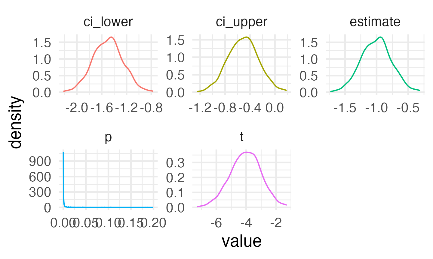

Distribution of results from simulated paired samples data

alpha <- 0.05
power <- mean(mysim_p$p < alpha)
power
## [1] 0.983

Intercept model

Now I’m going to show you a different way to simulate the same design. This might seem excessively complicated, but you will need this pattern when you start simulating data for mixed effects models.

Parameters

Remember, we used the following parameters to set up our simulation above:

sub_n  <- 100
A_mean <- 10
B_mean <- 11
A_sd   <- 2.5
B_sd   <- 2.5
AB_r   <- 0.5

From these, we can calculate the grand intercept (the overall mean regardless of condition), and the effect of condition (the mean of B minus A).

grand_i   <- (A_mean + B_mean)/2
AB_effect <- B_mean - A_mean

We also need to think about variance a little differently. First, calculate the pooled variance as the mean of the variances for A and B (remember, variance is SD squared).

pooled_var <- (A_sd^2 + B_sd^2)/2

The variance of the subject intercepts is r times this pooled variance and the error variance is what is left over. We take the square root (sqrt()) to set the subject intercept and error SDs for simulation later.

sub_sd   <- sqrt(pooled_var * AB_r)
error_sd <- sqrt(pooled_var * (1-AB_r))

Subject intercepts

Now we use these variables to create a data table for our subjects. Each subject gets an ID and a random intercept (sub_i). The intercept is simulated from a random normal distribution with a mean of 0 and an SD of sub_sd. This represents how much higher or lower than the average score each subject tends to be (regardless of condition).

sub <- tibble(
  sub_id = 1:sub_n,
  sub_i = rnorm(sub_n, 0, sub_sd)
)

Observations

Next, set up a table where each row represents one observation. We’ll use one of my favourite functions for simulation: crossing(). This creates every possible combination of the listed factors (it works the same as expand.grid(), but the results are in a more intuitive order). Here, we’re using it to create a row for each subject in each condition, since this is a fully within-subjects design.

obs <- crossing(
  sub_id = 1:sub_n,
  condition = c("A", "B")
)

Calculate the score

Next, we join the subject table so each row has the information about the subject’s random intercept and then calculate the score. I’ve done it in a few steps below for clarity. The score is just the sum of:

• the overall mean (grand_i)
• the subject-specific intercept (sub_i)
• the effect (effect): the numeric code for condition (condition.e) multiplied by the effect of condition (AB_effect)
• the error term (simulated from a normal distribution with mean of 0 and SD of error_sd)

dat <- obs %>%
  left_join(sub, by = "sub_id") %>%
  mutate(
    condition.e = recode(condition, "A" = -0.5, "B" = 0.5),
    effect = AB_effect * condition.e,
    error = rnorm(nrow(.), 0, error_sd),
    score = grand_i + sub_i + effect + error
  )

Use get_params to check the data. With data in long format, you need to specify the columns that contain the id, dv, and within-id variables.

# check the data
faux::get_params(dat, 
                 id = "sub_id",
                 dv = "score",
                 within = "condition")
##     n var    A    B  mean   sd
## 1 100   A 1.00 0.59  9.68 2.40
## 2 100   B 0.59 1.00 10.33 2.58

You can use the following code to put the data table into a more familiar “wide” format.

dat_wide <- dat %>%
  select(sub_id, condition, score) %>%
  spread(condition, score)

Analyses

You can analyse the data with a paired-samples t-test from the wide format:

# paired-samples t-test from dat_wide
t.test(dat_wide$A, dat_wide$B, paired = TRUE)
## 
##  Paired t-test
## 
## data:  dat_wide$A and dat_wide$B
## t = -2.8648, df = 99, p-value = 0.005095
## alternative hypothesis: true mean difference is not equal to 0
## 95 percent confidence interval:
##  -1.0923496 -0.1983759
## sample estimates:
## mean difference 
##      -0.6453628

Or in the long format:

# paired-samples t-test from dat (long)
t.test(score ~ condition, dat, paired = TRUE)
## 
##  Paired t-test
## 
## data:  score by condition
## t = -2.8648, df = 99, p-value = 0.005095
## alternative hypothesis: true mean difference is not equal to 0
## 95 percent confidence interval:
##  -1.0923496 -0.1983759
## sample estimates:
## mean difference 
##      -0.6453628

You can analyse the data with ANOVA using the aov_4() function from afex. (Notice how the F-value is the square of the t-value above.)

# anova using afex::aov_4
aov <- afex::aov_4(score ~ (condition | sub_id), data = dat)

aov$anova_table
## Anova Table (Type 3 tests)
## 
## Response: score
##           num Df den Df    MSE      F      ges   Pr(>F)   
## condition      1     99 2.5373 8.2072 0.016676 0.005095 **
## ---
## Signif. codes:  0 '***' 0.001 '**' 0.01 '*' 0.05 '.' 0.1 ' ' 1

You can even analyse the data with a mixed effects model using the lmer function (the afex version gives you p-values, but the lme4 version does not).

# mixed effect model using afex::lmer
lmem <- afex::lmer(score ~ condition.e + (1 | sub_id), data = dat)

# displays a tidy table of the fixed effects
broom.mixed::tidy(lmem, effects = "fixed")
## # A tibble: 2 × 7
##   effect term        estimate std.error statistic    df  p.value
##   <chr>  <chr>          <dbl>     <dbl>     <dbl> <dbl>    <dbl>
## 1 fixed  (Intercept)   10.0       0.222     45.0   99.0 9.08e-68
## 2 fixed  condition.e    0.645     0.225      2.86  99.0 5.10e- 3

Simulate a dataset from an analysis

Simulate a dataset from the parameters of an analysis. We’ll use the built-in dataset mtcars to predict miles per gallon (mpg) from transmission type (am) and engine type (vs).

model <- lm(mpg ~ am * vs, data = mtcars)
broom::tidy(model)
## # A tibble: 4 × 5
##   term        estimate std.error statistic  p.value
##   <chr>          <dbl>     <dbl>     <dbl>    <dbl>
## 1 (Intercept)    15.0       1.00     15.0  6.34e-15
## 2 am              4.70      1.74      2.71 1.14e- 2
## 3 vs              5.69      1.65      3.45 1.80e- 3
## 4 am:vs           2.93      2.54      1.15 2.59e- 1

Simulate

We can now simulate a dataset with 50 observations from each transmission type (am) and engine type (vs) combination, then use the model parameters to generate predicted values for mpg.

err_sd <- sigma(model) # SD of the error term from the model
fx <- coefficients(model) # fixed effect coefficients

sim_mtcars <- tibble(
  am = rep(c(0, 0, 1, 1), each = 50),
  vs = rep(c(0, 1, 0, 1), each = 50)
) %>%
  mutate(err = rnorm(200, 0, err_sd),
         mpg = fx[1] + 
               fx["am"]*am + 
               fx["vs"]*vs +
               fx["am:vs"]*am*vs + err)
  

Analyse the simulated data with lm() and output the results as a table using broom::tidy()

sim_model <- lm(mpg ~ am * vs, data = sim_mtcars)
broom::tidy(sim_model)
## # A tibble: 4 × 5
##   term        estimate std.error statistic  p.value
##   <chr>          <dbl>     <dbl>     <dbl>    <dbl>
## 1 (Intercept)    14.8      0.523     28.3  3.18e-71
## 2 am              5.61     0.739      7.60 1.21e-12
## 3 vs              6.62     0.739      8.95 2.67e-16
## 4 am:vs           1.96     1.05       1.87 6.24e- 2

Function

carsim <- function(n, b0, b_am, b_vs, b_am_vs, err_sd) {
  sim_mtcars <- tibble(
    am = rep(c(0, 0, 1, 1), each = n),
    vs = rep(c(0, 1, 0, 1), each = n)
  ) %>%
    mutate(err = rnorm(n*4, 0, err_sd),
           mpg = b0 + b_am*am + b_vs*vs + b_am_vs*am*vs + err)
  
  sim_model <- lm(mpg ~ am * vs, data = sim_mtcars)
  broom::tidy(sim_model)
}

Run the function with the values from the original model, but cut the fixed effect sizes in half.

err_sd <- sigma(model)
fx2 <- coefficients(model)/2

carsim(50, fx2[1], fx2[2], fx2[3], fx2[4], err_sd)
## # A tibble: 4 × 5
##   term        estimate std.error statistic  p.value
##   <chr>          <dbl>     <dbl>     <dbl>    <dbl>
## 1 (Intercept)    7.25      0.535    13.5   6.06e-30
## 2 am             2.78      0.757     3.67  3.11e- 4
## 3 vs             3.97      0.757     5.25  3.95e- 7
## 4 am:vs         -0.200     1.07     -0.187 8.52e- 1

Repeat this 100 time and calculate power for each effect.

simstats <- map_df(1:100, ~carsim(50, fx2[1], fx2[2], fx2[3], fx2[4], err_sd))

simstats %>%
  group_by(term) %>%
  summarise(power = mean(p.value < .05), .groups = "drop")
## # A tibble: 4 × 2
##   term        power
##   <chr>       <dbl>
## 1 (Intercept)  1   
## 2 am           0.92
## 3 am:vs        0.3 
## 4 vs           0.96

Exercises

Using the dataset below, predict moral disgust from the interaction between pathogen and sexual disgust using lm().

disgust <- read_csv("https://psyteachr.github.io/msc-data-skills/data/disgust_scores.csv")
## Rows: 20000 Columns: 6
## ── Column specification ────────────────────────────────────────────────────────
## Delimiter: ","
## dbl  (5): id, user_id, moral, pathogen, sexual
## date (1): date
## 
## ℹ Use `spec()` to retrieve the full column specification for this data.
## ℹ Specify the column types or set `show_col_types = FALSE` to quiet this message.

Simulate a new dataset of 100 people with a similar pathogen and sexual disgust distribution to the original dataset. Remember that these are likely to be correlated and that scores can only range from 0 to 6. (Hint: look at the help for norm2trunc)

Write a function to simulate data, analyse it, and return a table of results. Make sure you can vary the important parameters using arguments.

Calculate power for the same fixed effects as in the original analysis. Adjust the N until the dsign has around .80 power to detect a main effect of pathogen disgust.