Experimentum Data Wrangling Demo
(updated 2021-01-21)
Experimentum studies require that you download data from questionnaires and experiments separately, since the data have different formats. You can participate anonymously in the demo study (the median completion time is 3.8 minutes). The links below update dynamically, so your data will be available immediately.
The project structure file above is a JSON-formatted file that contains all of the information needed to run a study in Experimentum. In future versions of Experimentum, you will be able to directly edit this file, for example translating the questions into another language, and set up a study by simply uploading the file.
proj <- jsonlite::read_json("data/project_520_structure.json")Questionnaire Data
The study has two questionnaires: Groups, a few questions you can use to divide the participants into groups of varying sizes, and BMIS, the Brief Mood Introspection Scale.
Load Data
quest_data <- read_csv("data/Demo-Data-quests_2021-01-21.csv")

glimpse(quest_data)
## Rows: 2,807
## Columns: 14
## $ session_id <dbl> 60481, 60481, 60481, 60481, 60481, 60481, 60481, 60481, 60…
## $ project_id <dbl> 520, 520, 520, 520, 520, 520, 520, 520, 520, 520, 520, 520…
## $ quest_name <chr> "Groups", "Groups", "Groups", "Groups", "Groups", "Groups"…
## $ quest_id <dbl> 2921, 2921, 2921, 2921, 2921, 2921, 2921, 2920, 2920, 2920…
## $ user_id <dbl> 43533, 43533, 43533, 43533, 43533, 43533, 43533, 43533, 43…
## $ user_sex <chr> "female", "female", "female", "female", "female", "female"…
## $ user_status <chr> "res", "res", "res", "res", "res", "res", "res", "res", "r…
## $ user_age <dbl> 26.6, 26.6, 26.6, 26.6, 26.6, 26.6, 26.6, 26.6, 26.6, 26.6…
## $ q_name <chr> "fiber_arts", "native_english", "hats", "pets", "colour", …
## $ q_id <dbl> 92833810, 92833809, 92833814, 92833811, 92833813, 92833815…
## $ order <dbl> 1, 2, 3, 4, 5, 6, 7, 1, 2, 3, 4, 5, 6, 7, 8, 9, 10, 11, 12…
## $ dv <chr> "1", "0", "5", "Yes", "Red", "1", "today", "2", "1", "2", …
## $ starttime <dttm> 2021-01-19 17:48:15, 2021-01-19 17:48:15, 2021-01-19 17:4…
## $ endtime <dttm> 2021-01-19 17:48:31, 2021-01-19 17:48:31, 2021-01-19 17:4…session_ida unique ID generated each time someone starts a studyproject_ida unique ID for this studyquest_namethe name of each questionnaire (not guaranteed to be unique)quest_iduniquely identifies each questionnaireuser_idregistered participants have a unique ID that is the same across logins, while guest participants get a new ID each time they log inuser_sexgender from the options “male”, “female”, “nonbinary”, “na” (specifically chose not to answer), orNA(did not complete the question)user_statuswhether use is a researcher (“admin”, “super”, “res”, “student”), a “registered” user, a “guest” user, or “test”user_agethe user’s age; registered accounts are asked for their birthdate, and their age is calculated to the nearest 0.1 years; guest users may be asked their age in yearsq_namename of the questionq_iduniquely identifies each questionorderthe order the question was presented in (not necessarily answered in) or questionnaires with randomised orderdvthe responsestarttimethe time that the questionnaire was startedendtimethe time that the questionnaire was submitted
Removing duplicate answers
Although Experimentum tries to prevent people accidentally using the back button during a study, there are some ways around this, so sometimes a person will submit the same questionnaire twice in a row. You can filter your data down to only the first time each person completed each question with the following code (do not use this if your study actually gives people the same questionnaire more than once).
The questions are recorded in the order that they were answered, so we can just group by participant (user_id) and question (q_id) and choose the first answer. If you have a longitudinal study, group by session_id to allow multiple sessions per user.
quest_distinct <- quest_data %>%
  group_by(user_id, q_id) %>% # or add session_id
  # chooses the first time each user answered each question
  filter(row_number() == 1) %>%
  ungroup()
Check how many duplicate rows were excluded.
setdiff(quest_data, quest_distinct) %>% nrow()## [1] 0Groups
Here, we select just the data from the Groups questionnaire and keep only the session_id, user_id, q_name, and dv columns, and convert the data to wide format. If you restricted your data to only one session per user, as above, then user_id and session_id are redundant. The code below works for both types of data, though.
If the dv column contains both numeric and character data, the new columns will all be characters, so add convert = TRUE if you are using spread(). If you use the pivot_wider() function, it doesn’t have a convert argument, so you have to pipe the data frame to a separate function, type.convert().
groups <- quest_distinct %>%
  filter(quest_name == "Groups") %>%
  select(session_id, user_id, q_name, dv) %>%
spread(q_name, dv, convert = TRUE)| session_id | user_id | colour | exercise | fiber_arts | hats | native_english | pets | spiders |
|---|---|---|---|---|---|---|---|---|
| 60481 | 43533 | Red | today | 1 | 5 | 0 | Yes | 1 |
| 60495 | 31625 | Green | today | 1 | 3 | 1 | Yes | 5 |
| 60509 | 53422 | black | more | 0 | 5 | 1 | Yes | 2 |
| 60550 | 53458 | purplE | today | 1 | 12 | 1 | No | 3 |
| 60552 | 53460 | green | today | 0 | 3 | 0 | No | 2 |
| 60553 | 53461 | Blue | today | 0 | 5 | 1 | Yes | 2 |
Questionnaire options
I usually recommend recording the actual text chosen from drop-down menus, rather than integers that you will have to remember how you mapped onto the answers. If you need to check how you set up the coding, you can look at the info page on Experimentum or check the project json file that we loaded above. It’s a nested list and contains all the info, but can be a little tricky to parse (I’ll work on making an R package to make this easier in the future).
# get question names, text and type, plus options if select
qs <- proj$quest_2921$question %>%
  map(~{
    x <- .x[c("name", "question", "type")]
    if (!is.null(.x$options)) {
      x$options <- sapply(.x$options, `[[`, "display")
      names(x$options) <- sapply(.x$options, `[[`, "opt_value")
    }
    x
})- name: native_english
- question: Is English your native language?
- type: select
- options:
- 1: Yes
- 0: No
- name: fiber_arts
- question: Do you know how to knit or crochet?
- type: select
- options:
- 1: Yes
- 0: No
- name: pets
- question: Do you have a pet?
- type: select
- options:
- Yes: Yes
- No: No
- name: exercise
- question: When was the last time you exercised?
- type: select
- options:
- today: today or yesterday
- week: in the past week
- more: more than a week ago
- name: colour
- question: What is your favourite colour?
- type: text
- name: hats
- question: How many hats do you own (approximately)?
- type: selectnum
- name: spiders
- question: Are you afraid of spiders?
- type: radioanchor
Plots and tables
Plot your data or create summary tables to help you spot any problems. The count() function is useful for variables with a small number of options.
# count a single column
count(groups, exercise)| exercise | n |
|---|---|
| more | 24 |
| today | 69 |
| week | 31 |
# count multiple columns
count(groups, fiber_arts, native_english, pets)| fiber_arts | native_english | pets | n |
|---|---|---|---|
| 0 | 0 | No | 10 |
| 0 | 0 | Yes | 8 |
| 0 | 1 | No | 20 |
| 0 | 1 | Yes | 20 |
| 1 | 0 | No | 4 |
| 1 | 0 | Yes | 5 |
| 1 | 1 | No | 18 |
| 1 | 1 | Yes | 39 |
Histograms or density plots are best for columns with many continuous values.
ggplot(groups, aes(hats)) +
  geom_histogram(binwidth = 1,
                 fill = "dodgerblue",
                 color = "white")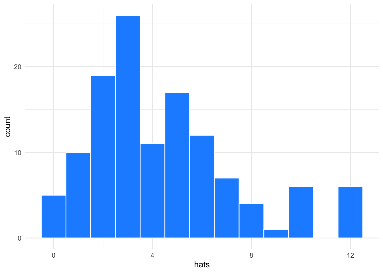
ggplot(groups, aes(spiders)) +
  geom_histogram(binwidth = 1,
                 fill = "violetred",
                 color = "white")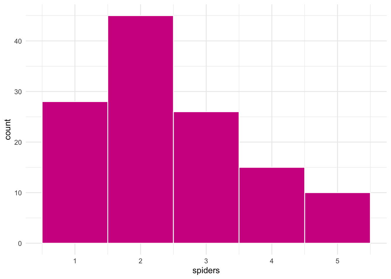
Recode variables
You might want to do some recoding of variables here. The pets column contains the words “Yes” and “No”; maybe you want to code this as 1s and 0s.The column fiber_arts has a 1 if a person knows how to knit or crochet, and a 0 if they don’t. You might want to change this to the words “Yes” and “No”. The recode() function is useful for this. I like to give the binary-coded version of a variable the suffix “.b”.
Note that in the recode() function, numbers that are on the left side of an equal sign need to be in quotes. This just has to do with the way R treats argument names and doesn’t mean that the recoded column has to be a character type.
groups_coded <- groups %>%
  mutate(
    pets.b = recode(pets, "Yes" = 1, "No" = 0),
    fiber_arts.b = fiber_arts,
    fiber_arts = recode(fiber_arts, "1" = "Yes", "0" = "No")
)| session_id | user_id | colour | exercise | fiber_arts | hats | native_english | pets | spiders | pets.b | fiber_arts.b |
|---|---|---|---|---|---|---|---|---|---|---|
| 60481 | 43533 | Red | today | Yes | 5 | 0 | Yes | 1 | 1 | 1 |
| 60495 | 31625 | Green | today | Yes | 3 | 1 | Yes | 5 | 1 | 1 |
| 60509 | 53422 | black | more | No | 5 | 1 | Yes | 2 | 1 | 0 |
| 60550 | 53458 | purplE | today | Yes | 12 | 1 | No | 3 | 0 | 1 |
| 60552 | 53460 | green | today | No | 3 | 0 | No | 2 | 0 | 0 |
| 60553 | 53461 | Blue | today | No | 5 | 1 | Yes | 2 | 1 | 0 |
Free text
If you have any free-text responses, you will probably need to code them. I always start by looking at all of the possible values after transforming the value to lowercase and getting rid of spaces around the text.
colours <- groups_coded %>%
  mutate(colour = tolower(colour) %>% trimws()) %>%
  count(colour) %>%
  arrange(n, colour) %>%
  group_by(n) %>%
  summarise(colours = paste(colour, collapse = ", "),
.groups = "drop")| n | colours |
|---|---|
| 1 | amber, cornflower, grey, indian orange, magenta, monochrome grey/white tones, petroleum blue, teal, violet, white, yes. |
| 4 | pink, turquoise |
| 6 | orange |
| 7 | black |
| 8 | yellow |
| 12 | red |
| 17 | purple |
| 26 | green |
| 29 | blue |
You can then decide to recode some colours to fix misspellings, etc. One tricky part of using recode() is that all replaced values have to be the same data type, so use NA_character_ if you are replacing values with strings, NA_real_ for doubles, and NA_integer_ for integers.
groups_colours <- groups_coded %>%
  mutate(colour = tolower(colour) %>% trimws()) %>%
  mutate(colours_fixed = recode(colour,
                                "amber" = "yellow",
                                "yes." = NA_character_,
                                "violet" = "purple",
                                "petroleum blue" = "blue"))
BMIS
The second questionnaire is the Brief Mood Introspection Scale (BMIS). The BMIS has 16 questions divided into positive and negative adjectives. The question names are all in the format valence_adjective, so you can easily separate the question name into two columns.
Because the original quest_data had both character and numeric values in the dv column, it is still a character type even now that the dv column only contains numbers. You can fix this using the type_convert() function. Set col_types manually or use cols() to automatically guess.
bmis_raw <- quest_distinct %>%
  filter(quest_name == "BMIS") %>%
  select(session_id, user_id, q_name, dv) %>%
  separate(q_name, c("valence", "adjective")) %>%
type_convert(col_types = cols())| session_id | user_id | valence | adjective | dv |
|---|---|---|---|---|
| 60481 | 43533 | neg | nervous | 2 |
| 60481 | 43533 | pos | caring | 1 |
| 60481 | 43533 | pos | peppy | 2 |
| 60481 | 43533 | neg | tired | 3 |
| 60481 | 43533 | neg | grouchy | 4 |
| 60481 | 43533 | neg | sad | 3 |
Summary scores
The BMIS is coded as the sum of the forward-coded scores for all the positive adjectives and the reverse-coded scores for all negative adjectives. Experimentum has a function to reverse code selected items in the “radiopage” questionnaire type, but we didn’t do that here so you can see how to manually recode. The scores are 1 to 4, so subjtract them from 5 to get the reverse-coded value. Make sure to look at a few of your recoded values to make sure it’s doing what you expect.
bmis_coded <- bmis_raw %>%
  mutate(recoded_dv = case_when(
    valence == "pos" ~ dv,
    valence == "neg" ~ 5 - dv
))| session_id | user_id | valence | adjective | dv | recoded_dv |
|---|---|---|---|---|---|
| 60481 | 43533 | neg | nervous | 2 | 3 |
| 60481 | 43533 | pos | caring | 1 | 1 |
| 60481 | 43533 | pos | peppy | 2 | 2 |
| 60481 | 43533 | neg | tired | 3 | 2 |
| 60481 | 43533 | neg | grouchy | 4 | 1 |
| 60481 | 43533 | neg | sad | 3 | 2 |
Create the summary score by grouping by user_id and session_id and summing the responses. We use sum() here because the BMIS is not valid if people skipped any questions, so we want the result to be NA if they did. Some questionnaire scoring allows you to calculate an average score omitting missed questions, so you could use mean(recoded_dv, na.rm = TRUE).
bmis <- bmis_coded %>%
  group_by(session_id, user_id) %>%
  summarise(bmis = sum(recoded_dv),
            .groups = "drop")
Plots
Always plot your summary scores. This helps you to double-check your logic and identify outliers.
ggplot(bmis, aes(bmis)) +
  geom_histogram(binwidth = 1,
                 fill = "dodgerblue",
                 color = "white")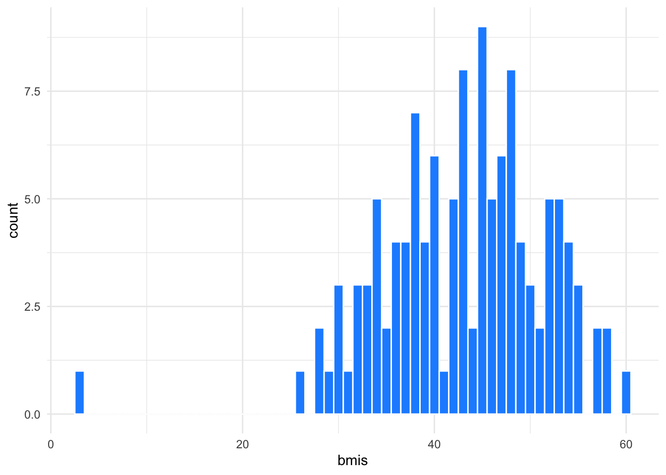
User Demographics
Experimentum data always contains user demographic data, which is collected when the user signs up for a registered account or logs in as a guest. This study did not ask users for their age or sex, so that info is only available from registered users.
First, we select the session_id and all of the user variables, then make sure we have only one row for each participant.
user <- quest_distinct %>%
  select(session_id, starts_with("user_")) %>%
distinct()| session_id | user_id | user_sex | user_status | user_age |
|---|---|---|---|---|
| 60481 | 43533 | female | res | 26.6 |
| 60495 | 31625 | female | student | 22.1 |
| 60509 | 53422 | female | guest | 61.0 |
| 60550 | 53458 | NA | guest | 0.0 |
| 60552 | 53460 | NA | guest | 0.0 |
| 60553 | 53461 | NA | guest | 0.0 |
Rejoining
Now you can rejoin your questionnaire data. Start with the user table and only join on matching data from the individual questionnaires. Use session_id and user_id to join.
q_data <- user %>%
  left_join(bmis, by = c("session_id", "user_id")) %>%
  left_join(groups_colours, by = c("session_id", "user_id"))
Exclusions
You will usually want to exclude participants with user_status that are not “registered” or “guest”. Statuses “admin”, “super”, “res”, and “student” refer to different types of researchers (with different privileges on the Experimentum platform). The status “test” is for test runs with different user demographics. You can also apply other exclusion criteria here like age restrictions or requiring that summary score not be missing.
q_data_excl <- q_data %>%
filter(user_status %in% c("guest", "registered"))| user_status | n |
|---|---|
| guest | 121 |
Experiment Data
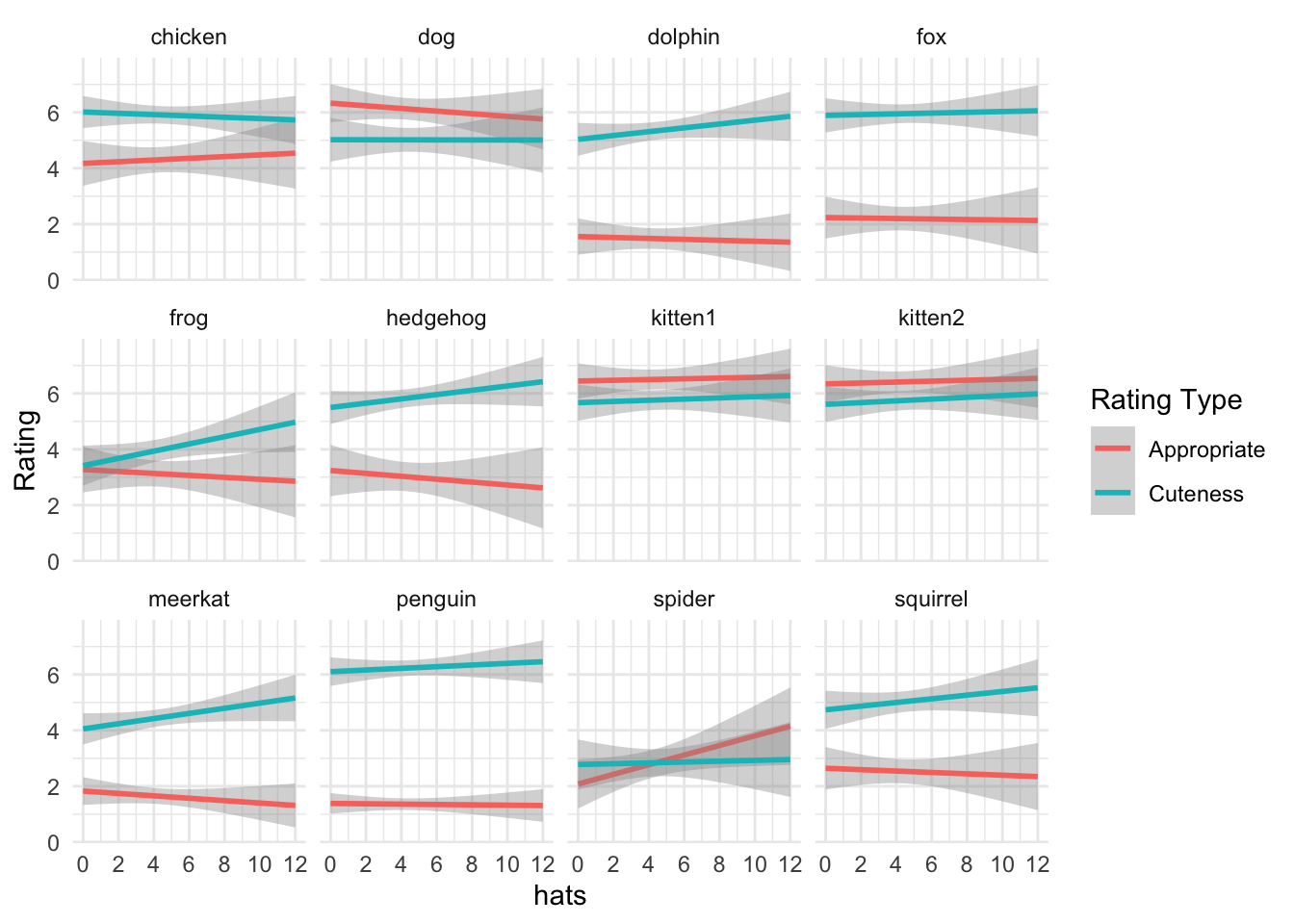
Our study has one rating experiment with two between-subject conditions: cuteness ratings and appropriateness as pet ratings.
Load Data
exp_data <- read_csv("data/Demo-Data-exps_2021-01-21.csv")

glimpse(exp_data)
## Rows: 1,476
## Columns: 15
## $ session_id <dbl> 60481, 60481, 60481, 60481, 60481, 60481, 60481, 60481, 60…
## $ project_id <dbl> 520, 520, 520, 520, 520, 520, 520, 520, 520, 520, 520, 520…
## $ exp_name <chr> "Animals: Cuteness", "Animals: Cuteness", "Animals: Cutene…
## $ exp_id <dbl> 707, 707, 707, 707, 707, 707, 707, 707, 707, 707, 707, 707…
## $ user_id <dbl> 43533, 43533, 43533, 43533, 43533, 43533, 43533, 43533, 43…
## $ user_sex <chr> "female", "female", "female", "female", "female", "female"…
## $ user_status <chr> "res", "res", "res", "res", "res", "res", "res", "res", "r…
## $ user_age <dbl> 26.6, 26.6, 26.6, 26.6, 26.6, 26.6, 26.6, 26.6, 26.6, 26.6…
## $ trial_name <chr> "animal-967657_640", "surprised-3786845_640", "penguins-42…
## $ trial_n <dbl> 2, 12, 9, 3, 8, 10, 5, 6, 7, 11, 4, 1, 4, 10, 7, 11, 12, 9…
## $ order <dbl> 1, 2, 3, 4, 5, 6, 7, 8, 9, 10, 11, 12, 1, 2, 3, 4, 5, 6, 7…
## $ dv <dbl> 7, 7, 7, 7, 7, 7, 7, 7, 7, 7, 7, 7, 1, 7, 7, 3, 4, 2, 7, 4…
## $ rt <dbl> 1756, 1103, 842, 735, 755, 845, 878, 842, 812, 1421, 1003,…
## $ side <dbl> 1, 1, 1, 1, 1, 1, 1, 1, 1, 1, 1, 1, 1, 1, 1, 1, 1, 1, 1, 1…
## $ dt <dttm> 2021-01-19 17:48:35, 2021-01-19 17:48:36, 2021-01-19 17:4…Experiment data have the same session and user columns as questionnaire data, plus columns for the experiment name (exp_name) and unique id (exp_id). The remaining columns give data specific to each trial:
trial_namenot necessarily uniquetrial_nuniquely identifies each trial within an experimentorder(the order the trial was shown to that participantdvthe responsertthe rough reaction time in milliseconds (web data have many sources of possible bias so do not use Experimentum to do RT experiments that require millisecond precision)sideif the experiment has multiple images, the order of the images if side is set to random (not relevant here)dtthe timestamp of the response
glimpse(exp_data)## Rows: 1,476
## Columns: 15
## $ session_id <dbl> 60481, 60481, 60481, 60481, 60481, 60481, 60481, 60481, 60…
## $ project_id <dbl> 520, 520, 520, 520, 520, 520, 520, 520, 520, 520, 520, 520…
## $ exp_name <chr> "Animals: Cuteness", "Animals: Cuteness", "Animals: Cutene…
## $ exp_id <dbl> 707, 707, 707, 707, 707, 707, 707, 707, 707, 707, 707, 707…
## $ user_id <dbl> 43533, 43533, 43533, 43533, 43533, 43533, 43533, 43533, 43…
## $ user_sex <chr> "female", "female", "female", "female", "female", "female"…
## $ user_status <chr> "res", "res", "res", "res", "res", "res", "res", "res", "r…
## $ user_age <dbl> 26.6, 26.6, 26.6, 26.6, 26.6, 26.6, 26.6, 26.6, 26.6, 26.6…
## $ trial_name <chr> "animal-967657_640", "surprised-3786845_640", "penguins-42…
## $ trial_n <dbl> 2, 12, 9, 3, 8, 10, 5, 6, 7, 11, 4, 1, 4, 10, 7, 11, 12, 9…
## $ order <dbl> 1, 2, 3, 4, 5, 6, 7, 8, 9, 10, 11, 12, 1, 2, 3, 4, 5, 6, 7…
## $ dv <dbl> 7, 7, 7, 7, 7, 7, 7, 7, 7, 7, 7, 7, 1, 7, 7, 3, 4, 2, 7, 4…
## $ rt <dbl> 1756, 1103, 842, 735, 755, 845, 878, 842, 812, 1421, 1003,…
## $ side <dbl> 1, 1, 1, 1, 1, 1, 1, 1, 1, 1, 1, 1, 1, 1, 1, 1, 1, 1, 1, 1…
## $ dt <dttm> 2021-01-19 17:48:35, 2021-01-19 17:48:36, 2021-01-19 17:4…Most researchers don’t want all that data, so we can select just the important columns. The exp_name contains info we don’t need, so we’ll also process that.
exp_selected <- exp_data %>%
  select(session_id, user_id, exp_name, trial_name, dv) %>%
  mutate(exp_name = sub("Animals: ", "", exp_name))
count(exp_selected, exp_name)| exp_name | n |
|---|---|
| Appropriate | 696 |
| Cuteness | 780 |
count(exp_selected, trial_name)| trial_name | n |
|---|---|
| adorable-5059091_640 | 123 |
| animal-967657_640 | 123 |
| bird-349035_640 | 123 |
| dolphin-203875_640 | 123 |
| frog-3312038_640 | 123 |
| hedgehog-468228_640 | 123 |
| kitty-2948404_640 | 123 |
| meerkat-459171_640 | 123 |
| penguins-429134_640 | 123 |
| pug-690566_640 | 123 |
| spider-2313079_640 | 123 |
| surprised-3786845_640 | 123 |
Adding trial data
It’s common that you need to add some data about each trial.


Figure 1: images from the experiment
You will probably have you trial information in a separate table, so you can load that here. In this case, we’ll use the tribble() function to create a table by rows.
trial_info <- tribble(
  ~photo,                  ~name,    ~is_baby, ~mammal,
  "adorable-5059091_640",  "kitten1",   1,        1,
  "animal-967657_640",     "fox",       0,        1,
  "bird-349035_640",       "chicken",   1,        0,
  "dolphin-203875_640",    "dolphin",   0,        1,
  "frog-3312038_640",      "frog",      0,        0,
  "hedgehog-468228_640",   "hedgehog",  0,        1,
  "kitty-2948404_640",     "kitten2",   1,        1,
  "meerkat-459171_640",    "meerkat",   0,        1,
  "penguins-429134_640",   "penguin",   1,        0,
  "pug-690566_640",        "dog",       1,        1,
  "spider-2313079_640",    "spider",    0,        0,
  "surprised-3786845_640", "squirrel",  0,        1
)
Then you can join it to the experiment data.
exp_full <- exp_selected %>%
  left_join(trial_info, by = c("trial_name" = "photo"))
And create some plots.
ggplot(exp_full, aes(dv, colour = exp_name)) +
  geom_freqpoly(binwidth = 1) +
  facet_wrap(~name) +
  scale_x_continuous(breaks = 1:7) +
  labs(colour = "Rating Type", x = "")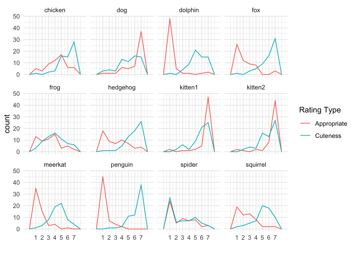
Demographs, exclusions and rejoin
As for the questionnaire data above, you can pull out the user demographics, apply exclusions, and rejoin to the experiment data.
# user table with exclusions
user_excl <- exp_data %>%
  select(session_id, starts_with("user_")) %>%
  distinct() %>%
  filter(user_status %in% c("guest", "registered"))

e_data_excl <- user_excl %>%
left_join(exp_full, by = c("session_id", "user_id"))glimpse(e_data_excl)## Rows: 1,440
## Columns: 11
## $ session_id <dbl> 60509, 60509, 60509, 60509, 60509, 60509, 60509, 60509, 60…
## $ user_id <dbl> 53422, 53422, 53422, 53422, 53422, 53422, 53422, 53422, 53…
## $ user_sex <chr> "female", "female", "female", "female", "female", "female"…
## $ user_status <chr> "guest", "guest", "guest", "guest", "guest", "guest", "gue…
## $ user_age <dbl> 61, 61, 61, 61, 61, 61, 61, 61, 61, 61, 61, 61, 0, 0, 0, 0…
## $ exp_name <chr> "Appropriate", "Appropriate", "Appropriate", "Appropriate"…
## $ trial_name <chr> "penguins-429134_640", "bird-349035_640", "hedgehog-468228…
## $ dv <dbl> 1, 4, 5, 1, 7, 1, 7, 6, 1, 7, 1, 1, 4, 4, 4, 4, 4, 4, 4, 4…
## $ name <chr> "penguin", "chicken", "hedgehog", "squirrel", "kitten2", "…
## $ is_baby <dbl> 1, 1, 0, 0, 1, 0, 1, 0, 0, 1, 0, 0, 1, 1, 0, 1, 0, 0, 1, 0…
## $ mammal <dbl> 0, 0, 1, 1, 1, 1, 1, 0, 1, 1, 1, 0, 1, 1, 0, 1, 1, 1, 0, 1…Joining Questionnaire and Experiment Data
Often, it makes most sense to process questionnaire data in wide format and experiment data in long format. If you need to add wide questionnaire data to a long experiment table, left join the questionnaire like this:
all_data <- e_data_excl %>%
  left_join(q_data_excl, by = c("session_id", "user_id"))

names(all_data)
## [1] "session_id" "user_id" "user_sex.x" "user_status.x"
## [5] "user_age.x" "exp_name" "trial_name" "dv"
## [9] "name" "is_baby" "mammal" "user_sex.y"
## [13] "user_status.y" "user_age.y" "bmis" "colour"
## [17] "exercise" "fiber_arts" "hats" "native_english"
## [21] "pets" "spiders" "pets.b" "fiber_arts.b"
## [25] "colours_fixed"Now go explore your data!
Lisa DeBruine
Professor of Psychology
Lisa DeBruine is a professor of psychology at the University of Glasgow. Her substantive research is on the social perception of faces and kinship. Her meta-science interests include team science (especially the Psychological Science Accelerator), open documentation, data simulation, web-based tools for data collection and stimulus generation, and teaching computational reproducibility.