Data from Images
I saw this a few days ago and sympathised, because I’ve often wanted to use data that is trapped in images or PDFs. If it’s not too much, I’ll manually transcribe it, but that’s so tedious!
crucial data being published as images … 😭😭😭😭 https://t.co/9CKg9NhYtA
— Shel 🇰🇪 (@Shel_Kariuki) October 15, 2021
A tweet by Abiyu Giday reminded me that the magick package has OCR (optical character recognition), so I decided to try it out.
Required packages
library(magick)    # for image processing
library(tesseract) # for OCR image reading
library(dplyr)     # for data wrangling and pipes
library(tidyr)     # for data wrangling
library(stringr)   # for string manipulation
library(ggplot2)   # for plots
Read the image
First, you need to read in the image and convert it to text using two functions from the magick package.
I use ImageMagick for webmorph development, so had it installed previously. I’m not sure if installing the R package also sets up the ImageMagick installation. If you’re on a Windows machine, the easiest way is to use installr::install.imagemagick(). On a Mac, you can install it with Homebrew using brew install imagemagick@6.
Now You can read in the image with image_read() and run OCR on it with image_ocr(). If you haven’t installed the tesseract package yet, the second function will prompt you to.
# original image source:
# https://pbs.twimg.com/media/FBv8P8XXEBgCBvS?format=jpg&name=medium
imgtext <- magick::image_read("data_image.jpg") %>%
  magick::image_ocr()
Process the text
The result is a single character string that looks like this, so we’re going to need to do quite a bit of processing to get it into a tabular format.
rs
COUNTY VACCINES AL |

1. Nairobi 957,147 (31.4%) 25. Homa Bay 33,290 (5.5%)
2. Kiambu 298,723 (18.4%) 26. Migori 32,670 (5.9%)
3. Nakuru 170,684 (13.4%) 27. Kilifi 31,611 (4.0%)
4. Nyeri 134,166 (26.3%) 28. Kisii 30,204 (4.3%)
5. Murang’a 110,825 (16.4%) 29. Nyamira 29,142 (8.5%)
6. Machakos 100,671 (11.1%) 30. Busia 26,792 (5.8%)
7. Uasin Gishu 92,142 (13.3%) 31. Vihiga 25,172 (7.6%)
8. Kisumu 90,495 (13.8%) 32. Tharaka Nithi 24,386 (9.9%)
9. Mombasa 82,814 (10.3%) 33. Baringo 21,176 (6.2%)
10. Kirinyaga 81,233 (19.6%) 34. Bomet 20,885 (4.5%)
ll. Kajiado 75,960 (11.5%) 35. Elgeyo Marakwet 17,574 (7.2%)
12. Bungoma 66,688 (7.9%) 36. Kwale 17,185 (3.8%)
13. Meru 66,270 (7.0%) 37. Narok 15,410 (2.8%)
14. Kakamega 62,043 (6.3%) 38. Turkana 9,249 (2.0%)
15. Nyandarua 60,574 (16.1%) 39. West Pokot 8,207 (2.9%)
16. Laikipia 58,141 (19.0%) 40. Garissa 7,694 (1.9%)
17. Makueni 57,435 (9.8%) 41. Samburu 6,686 (4.6%)
18. Embu 56,082 (14.2%) 42. Mandera 6,220 (1.8%)
19. Trans Nzoia 45,228 (8.7%) 43. Isiolo 5,653 (4.2%)
20. Kitui 40,663 (6.5%) 44. Wajir 5,003 (1.5%)
21. Kericho 38,497 (7.6%) 45. Lamu 4,692 (5.6%)
22. Siaya 38,313 (7.1%) 46. Tana River 3,440 (2.3%)
23. Nandi 38,243 (7.8%) 47. Marsabit 2,953 ( 1.3%)
24. Taita Taveta 34,478 (16.2%)
First, I’ll get rid of the first three lines.
You need to put two backslashes before the "\\|" to mark it as a literal |, since | has a special meaning in regular expressions (it means “or”). This is called escaping the character. The combination "\n" represents a line break.
trimmed <- gsub("rs\nCOUNTY VACCINES AL \\|\n\n", "", imgtext)

trimmed
## [1] "1. Nairobi 957,147 (31.4%) 25. Homa Bay 33,290 (5.5%)\n2. Kiambu 298,723 (18.4%) 26. Migori 32,670 (5.9%)\n3. Nakuru 170,684 (13.4%) 27. Kilifi 31,611 (4.0%)\n4. Nyeri 134,166 (26.3%) 28. Kisii 30,204 (4.3%)\n5. Murang’a 110,825 (16.4%) 29. Nyamira 29,142 (8.5%)\n6. Machakos 100,671 (11.1%) 30. Busia 26,792 (5.8%)\n7. Uasin Gishu 92,142 (13.3%) 31. Vihiga 25,172 (7.6%)\n8. Kisumu 90,495 (13.8%) 32. Tharaka Nithi 24,386 (9.9%)\n9. Mombasa 82,814 (10.3%) 33. Baringo 21,176 (6.2%)\n10. Kirinyaga 81,233 (19.6%) 34. Bomet 20,885 (4.5%)\nll. Kajiado 75,960 (11.5%) 35. Elgeyo Marakwet 17,574 (7.2%)\n12. Bungoma 66,688 (7.9%) 36. Kwale 17,185 (3.8%)\n13. Meru 66,270 (7.0%) 37. Narok 15,410 (2.8%)\n14. Kakamega 62,043 (6.3%) 38. Turkana 9,249 (2.0%)\n15. Nyandarua 60,574 (16.1%) 39. West Pokot 8,207 (2.9%)\n16. Laikipia 58,141 (19.0%) 40. Garissa 7,694 (1.9%)\n17. Makueni 57,435 (9.8%) 41. Samburu 6,686 (4.6%)\n18. Embu 56,082 (14.2%) 42. Mandera 6,220 (1.8%)\n19. Trans Nzoia 45,228 (8.7%) 43. Isiolo 5,653 (4.2%)\n20. Kitui 40,663 (6.5%) 44. Wajir 5,003 (1.5%)\n21. Kericho 38,497 (7.6%) 45. Lamu 4,692 (5.6%)\n22. Siaya 38,313 (7.1%) 46. Tana River 3,440 (2.3%)\n23. Nandi 38,243 (7.8%) 47. Marsabit 2,953 ( 1.3%)\n24. Taita Taveta 34,478 (16.2%)\n"Split into rows
Since there are two rows of data on each row, I’ll convert all of the line breaks ("\n") into spaces and then split the result wherever there is 0 or 1 spaces (" ?"), followed by 1 or more digits ("[0-9]+"), followed by a full stop and a space ("\\. ").
split_base <- gsub("\n", " ", trimmed) %>%
  strsplit(" ?[0-9]+\\. ")
If you prefer stringr functions to base functions, you can do it this way:
split_stringr <- trimmed %>%
  stringr::str_replace("\n", " ") %>%
  stringr::str_split(" ?s[0-9]+\\. ")
Fix encoding errors
Make sure you look through all of your data at this point. The first time I did this, I didn’t notice that 11. got read in as ll., so line 21 didn’t split.
split_base[[1]][21]## [1] "Bomet 20,885 (4.5%) ll. Kajiado 75,960 (11.5%)"You can fix that by replacing "ll. " with "11. " before you split the data.
split_base <- trimmed %>%
  gsub("ll. ", "11. ", .) %>%
  gsub("\n", " ", .) %>%
  strsplit(" ?[0-9]+\\. ")
Tabular format
Now we need to get this into a tabular format. The objects split_base and split_stringr are 1-item lists where the first item contains the vector of our rows. The first row is blank (the content before the first split at 1.) so we have to omit that. The code below creates a data frame.
data1 <- data.frame(x = split_base[[1]][-1]) | x |
|---|
| Nairobi 957,147 (31.4%) |
| Homa Bay 33,290 (5.5%) |
| Kiambu 298,723 (18.4%) |
| Migori 32,670 (5.9%) |
| Nakuru 170,684 (13.4%) |
| Kilifi 31,611 (4.0%) |
Separate columns
Now we have to separate the columns out. There are several ways to do this. If you’re a regex wizard, you don’t need the rest of this tutorial, so I’m going to break it into smaller steps instead. Using gsub() to create new columns by replacing parts of the original column is a straightforward way (HT Tan Ho).
Create the county column by replacing all characters from the space before the first digit ([0-9]) plus any characters after that (.*) until the end of the string ($). Create the number column by replacing from the start of the string (^) plus any non-numbers ([^0-9]+) that follow it.
data2 <- data1 %>%
  mutate(county = gsub(" [0-9].*$", "", x),
number = gsub("^[^0-9]+", "", x))| x | county | number |
|---|---|---|
| Nairobi 957,147 (31.4%) | Nairobi | 957,147 (31.4%) |
| Homa Bay 33,290 (5.5%) | Homa Bay | 33,290 (5.5%) |
| Kiambu 298,723 (18.4%) | Kiambu | 298,723 (18.4%) |
| Migori 32,670 (5.9%) | Migori | 32,670 (5.9%) |
| Nakuru 170,684 (13.4%) | Nakuru | 170,684 (13.4%) |
| Kilifi 31,611 (4.0%) | Kilifi | 31,611 (4.0%) |
The county column looks fine, but the number column needs to be split into the number of vaccinations and the percent. Use the separate() function to split this column on the left parenthesis (remember to escape it).
data3 <- data2 %>%
  separate(col = number,
           into = c("number", "percent"),
           sep = "\\(",
extra = "drop") | x | county | number | percent |
|---|---|---|---|
| Nairobi 957,147 (31.4%) | Nairobi | 957,147 | 31.4%) |
| Homa Bay 33,290 (5.5%) | Homa Bay | 33,290 | 5.5%) |
| Kiambu 298,723 (18.4%) | Kiambu | 298,723 | 18.4%) |
| Migori 32,670 (5.9%) | Migori | 32,670 | 5.9%) |
| Nakuru 170,684 (13.4%) | Nakuru | 170,684 | 13.4%) |
| Kilifi 31,611 (4.0%) | Kilifi | 31,611 | 4.0%) |
Clean up the data
Now we just need to clean up some extra characters in the number and percent columns. Get rid of the comma in the number column and the percent sign and right parenthesis in the percent column (remember to escape the parenthesis).
data4 <- data3 %>%
  mutate(number = gsub(",", "", number),
         percent = gsub("%\\)", "", percent)) %>%
select(-x)| county | number | percent |
|---|---|---|
| Nairobi | 957147 | 31.4 |
| Homa Bay | 33290 | 5.5 |
| Kiambu | 298723 | 18.4 |
| Migori | 32670 | 5.9 |
| Nakuru | 170684 | 13.4 |
| Kilifi | 31611 | 4.0 |
Check data types
This looks good, but there is still a problem. We can’t do anything useful with this data set because the number and percent columns are actually still character data types.
summary(data4)## county number percent
## Length:47 Length:47 Length:47
## Class :character Class :character Class :character
## Mode :character Mode :character Mode :characterm <- mean(data4$number)## Warning in mean.default(data4$number): argument is not numeric or logical:
## returning NAConvert the number column to an integer and the percent column to a double.
data <- data4 %>%
  mutate(number = as.integer(number),
percent = as.double(percent))| county | number | percent |
|---|---|---|
| Nairobi | 957147 | 31.4 |
| Homa Bay | 33290 | 5.5 |
| Kiambu | 298723 | 18.4 |
| Migori | 32670 | 5.9 |
| Nakuru | 170684 | 13.4 |
| Kilifi | 31611 | 4.0 |
Now you’re ready to plot the data or use it in analyses.
ggplot(data, aes(x = number, y = percent)) +
  geom_point(color = "dodgerblue") +
  scale_x_continuous("Number of Vaccinated People",
                     breaks = seq(0, 1e6, 2e5),
                     labels = c(paste0(seq(0, 800, 200), "K"), "1M"),
                     limits = c(0, 1e6)) +
  scale_y_continuous("Percent of County",
                     breaks = seq(0, 40, 10),
                     labels = paste0(seq(0, 40, 10), "%")) +
  theme_bw()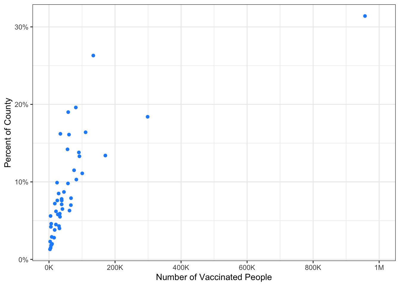
Glossary
| term | definition |
|---|---|
| character | A data type representing strings of text. |
| data type | The kind of data represented by an object. |
| double | A data type representing a real decimal number |
| escape | Include special characters like " inside of a string by prefacing them with a backslash. |
| integer | A data type representing whole numbers. |
| list | A container data type that allows items with different data types to be grouped together. |
| tabular data | Data in a rectangular table format, where each row has an entry for each column. |
| vector | A type of data structure that collects values with the same data type, like T/F values, numbers, or strings. |
Lisa DeBruine
Professor of Psychology
Lisa DeBruine is a professor of psychology at the University of Glasgow. Her substantive research is on the social perception of faces and kinship. Her meta-science interests include team science (especially the Psychological Science Accelerator), open documentation, data simulation, web-based tools for data collection and stimulus generation, and teaching computational reproducibility.