Mann-Whitney False Positives
One of my favourite colleagues, Phil McAleer, asked about unequal sample sizes for Mann-Whitney tests on our group chat today. I had no idea, so, as always, I thought “This is a job for simulations!”
I started by loading tidyverse, since I know I’ll need to wrangle data and plot things. I’m starting to get more comfortable with base R for package development, and it can make things faster, but tidyverse is my favourite for a quick analysis or a pipeline where understandability is more important than speed.
And I set my favourite seed so my simulations will give me a reproducible answer.
library(tidyverse)
set.seed(8675309)
Then I wrote a wee function to simulate data with the parameters I’m interested in varying, run a Mann-Whitney test, and return the p-value (all I need to look at power and false positives).
First, I just wanted to look at false positives for different sample size, so I set n1 and n2 as arguments and set alternative with a default of “two.sided”. The function wilcox.test runs a Mann-Whitney test for independent samples.
mw <- function(n1, n2, alternative = "two.sided") {
  x1 <- rnorm(n1)
  x2 <- rnorm(n2)
  w <- wilcox.test(x1, x2, alternative = alternative)
  w$p.value
}
Now I need to set up a table with all of the values I want to run simulations for. I set n1 and n2 to the numbers 10 to 100 in steps of ten. This was crossed with the number of replications I wanted to run (1000). I then removed the values where n2 > n1, since they’re redundant with the opposite version (e.g., n1 = 10, n2 = 20 is the same as n1 = 20, n2 = 10).
params <- expand.grid(
  n1 = seq(10, 100, 10),
  n2 = seq(10, 100, 10),
  reps = 1:1000
) %>%
filter(n1 <= n2)| n1 | n2 | reps |
|---|---|---|
| 10 | 10 | 1 |
| 10 | 20 | 1 |
| 20 | 20 | 1 |
| … | … | … |
| 80 | 100 | 1000 |
| 90 | 100 | 1000 |
| 100 | 100 | 1000 |
I then used the pmap_dbl function from purrr to map the values from n1 and n2 onto mw, then grouped the results by n1 and n2 and calculated false_pos as the proportion of p less than alpha.
alpha <- 0.05

mw1 <- params %>%
  mutate(p = pmap_dbl(list(n1, n2), mw)) %>%
  group_by(n1, n2) %>%
  summarise(false_pos = mean(p < alpha), .groups = "drop")
Then I plotted the false positive rate for each combination against the difference between n1 and n2. You can see that the false positive rate is approximately nominal, or equal to the specified alpha of 0.05.
ggplot(mw1, aes(n2 - n1, false_pos)) +
  geom_point(aes(color = as.factor(n1))) +
  geom_smooth(formula = y ~ x, method = lm, color = "black") +
  labs(x = "N2 - N1",
         y = "False Positive Rate",
         color = "N1") +
  ylim(0, .1)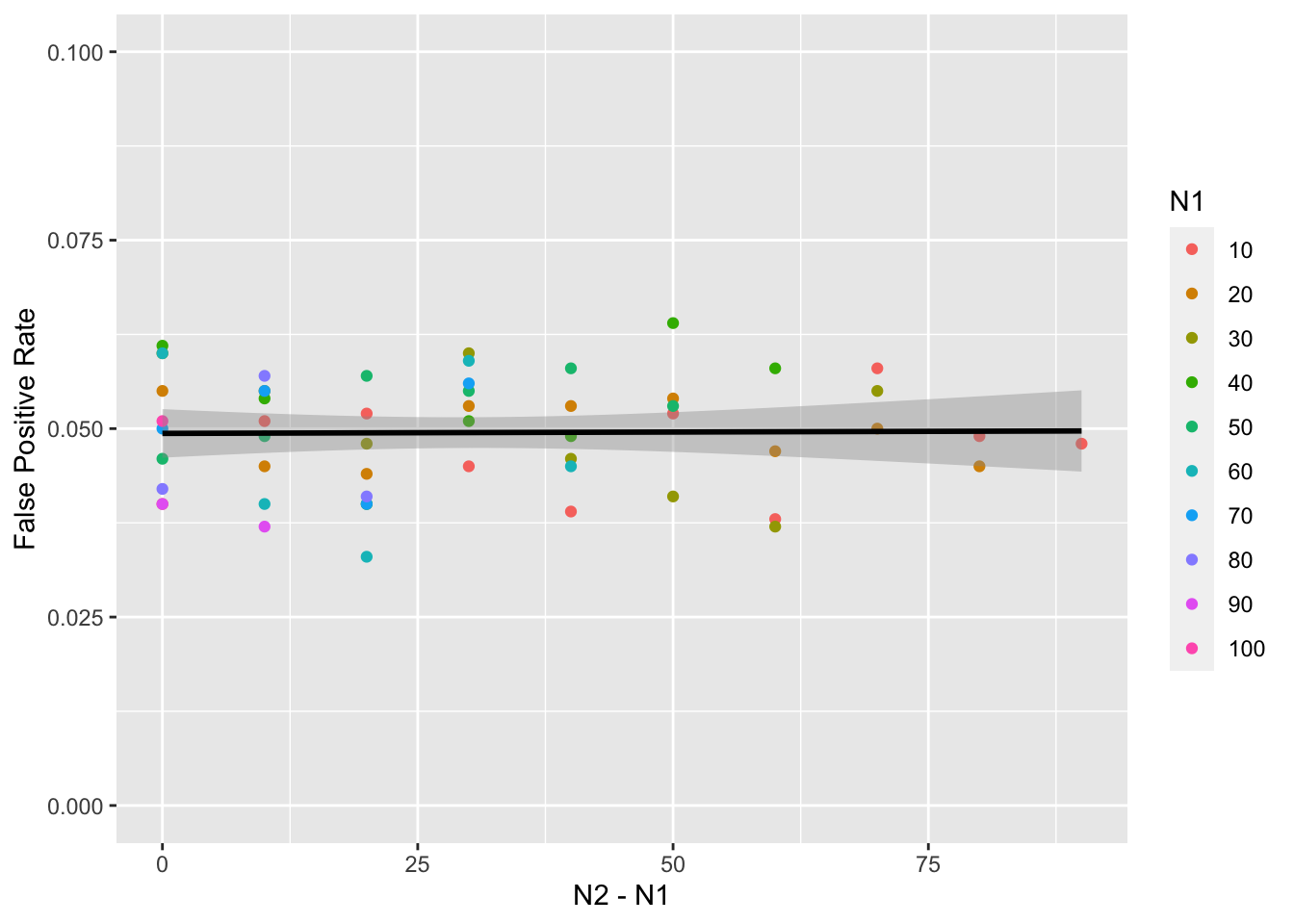
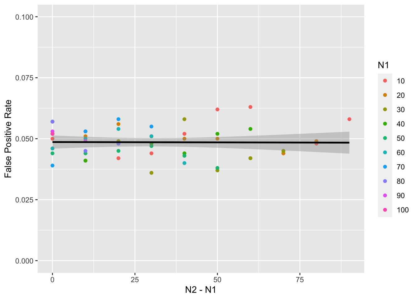
But what if data aren’t drawn from a normal distribution? We can change the mw() function to simulate data from a different distribtion, such as uniform, and run the whole process again.
mw <- function(n1, n2, alternative = "two.sided") {
  x1 <- runif(n1)
  x2 <- runif(n2)
  w <- wilcox.test(x1, x2, alternative = alternative)
  w$p.value
}
The rest of our code is identical to above.
mw2 <- params %>%
  mutate(p = pmap_dbl(list(n1, n2), mw)) %>%
  group_by(n1, n2) %>%
  summarise(false_pos = mean(p < alpha), .groups = "drop")
This doesn’t seem to make much difference.
What if the variance between the two samples is different? First, let’s adjust the mw() function to vary the SD of the two samples. We’ll give sd1 a default value of 1 and sd2 will default to the same as sd1. We might as well add the option to change the means, so default m1 to 0 and m2 to the same as m1.
mw <- function(n1, m1 = 0, sd1 = 1,
               n2 = n1, m2 = m1, sd2 = sd1,
               alternative = "two.sided") {
  x1 <- rnorm(n1, m1, sd1)
  x2 <- rnorm(n2, m2, sd2)
  w <- wilcox.test(x1, x2, alternative = alternative)
  w$p.value
}
Now we need to set up a new list of parameters to change. The Ns didn’t make much difference last time, so let’s vary them in steps of 20 this time. We’ll vary sd1 and sd2 from 0.5 to 2 in steps of 0.5, and also only keep combinations where sd1 is less than or equal to sd2 to avoid redundancy.
params <- expand.grid(
  reps = 1:1000,
  n1 = seq(10, 100, 20),
  n2 = seq(10, 100, 20),
  sd1 = seq(0.5, 2, 0.5),
  sd2 = seq(0.5, 2, 0.5)
) %>%
  filter(n1 <= n2, sd1 <= sd2)
mw3 <- params %>%
mutate(p = pmap_dbl(list(n1, 0, sd1, n2, 0, sd2), mw)) %>%
group_by(n1, n2, sd1, sd2) %>%
summarise(false_pos = mean(p < alpha), .groups = "drop")It looks like differences in SD make a big difference in the false positive rate, and the effect is bigger as Ns and SDs get more unequal.
ggplot(mw3, aes(sd2 - sd1, false_pos, color = as.factor(n2-n1))) +
  geom_point() +
  geom_smooth(formula = y ~ x, method = lm) +
  labs(x = "SD2 - SD1",
         y = "False Positive Rate",
         color = "N2-N1")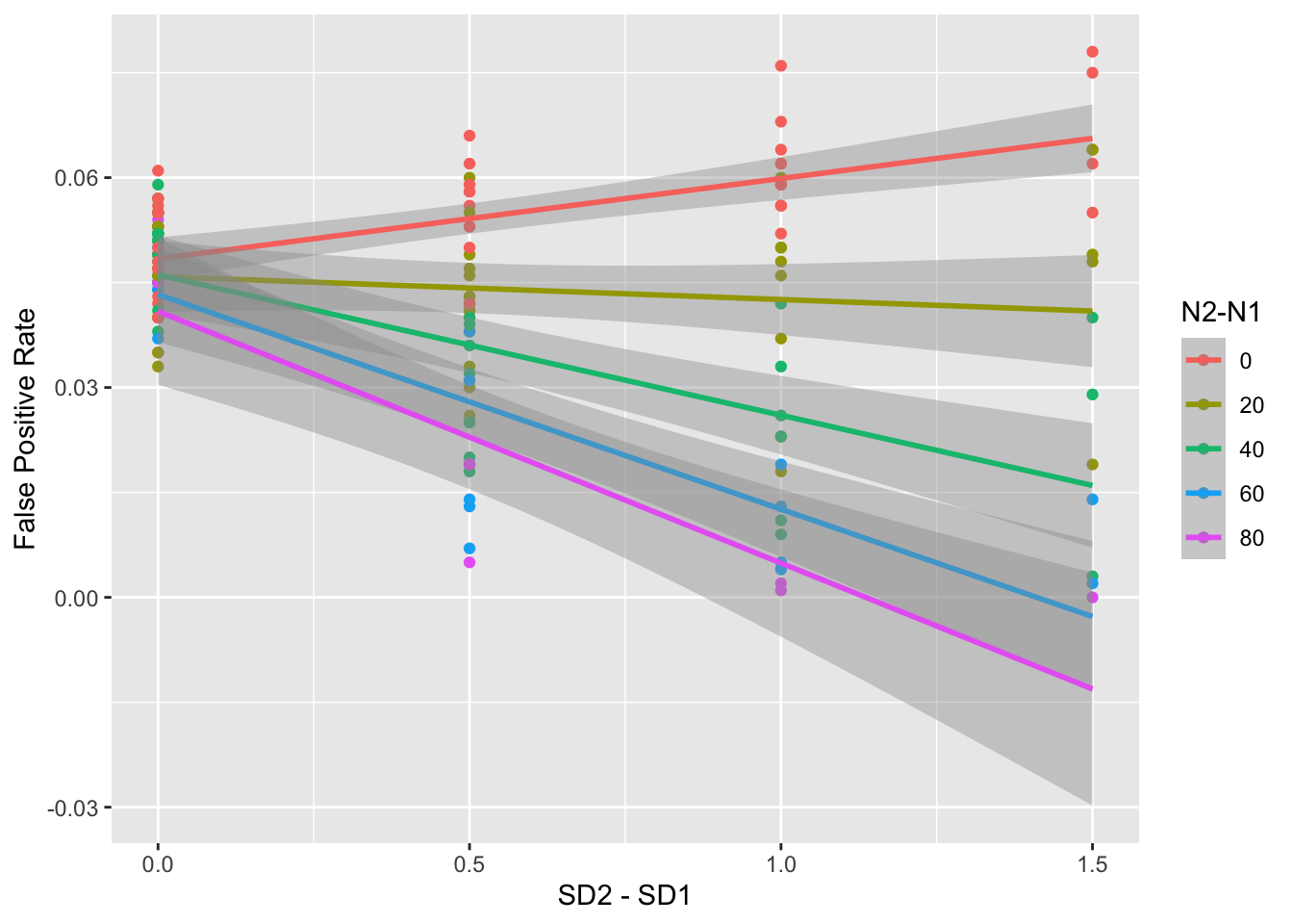
I’ll leave it to the enterprising reader to simulate power for different effect sizes.
Lisa DeBruine
Professor of Psychology
Lisa DeBruine is a professor of psychology at the University of Glasgow. Her substantive research is on the social perception of faces and kinship. Her meta-science interests include team science (especially the Psychological Science Accelerator), open documentation, data simulation, web-based tools for data collection and stimulus generation, and teaching computational reproducibility.