Inputting data table rows as function arguments
I was working on a simulation project with an undergraduate dissertation student today (I’m so amazed at what our students can do now!) and wanted to show her how to efficiently run simulations for all combinations of a range of parameters. It took 20 minutes of googling map functions in purrr to figure it out. I find I have to do this every time I want to use this pattern, so I decided to write a quick tutorial on it.
You’ll need functions from the purrr library, as well as some dplyr and tidyr functions, so I just load the whole tidyverse.
library(tidyverse)Fisrt, I need to define the function I want to run for the imulation. I’ll make a relatively simple one, that takes the samples sizes, means and standard deviations for two samples, simulates data, and returns the sample effect size, t-value, p-value, and degrees of freedom from t.test.
my_t_sim <- function(n1 = 100, m1 = 0, sd1 = 1,
                     n2 = 100, m2 = 0, sd2 = 1) {
  # simulate data
  grp1 <- rnorm(n1, m1, sd1)
  grp2 <- rnorm(n2, m2, sd2)

  # analyse
  tt <- t.test(grp1, grp2)

  # calculate cohens d for independent samples
  s_pooled <- sqrt(((n1-1) * sd(grp1)^2 + (n2-1) *
                      sd(grp2)^2)/(n1+n2))
  d <- (tt$estimate[[1]] - tt$estimate[[2]]) / s_pooled

  # return named list of values
  list(d = d,
       t  = tt$statistic[[1]],
       df = tt$parameter[[1]],
       p  = tt$p.value)
}
So we can simulate a study with 20 observations in each group and an effect size of 0.5.
my_t_sim(n1 = 20, m1 = 100, sd1 = 10,
         n2 = 20, m2 = 105, sd2 = 10)
## $d
## [1] -0.7037
##
## $t
## [1] -2.169
##
## $df
## [1] 33.89
##
## $p
## [1] 0.0372If you want to run it 100 times, you can use the map_df() function to create a data frame of the results for each repeat.
results <- map_df(1:100, ~my_t_sim(n1 = 20, m1 = 100, sd1 = 10,
n2 = 20, m2 = 105, sd2 = 10))| d | t | df | p |
|---|---|---|---|
| -0.6277 | -1.9346 | 34.22 | 0.0613 |
| -0.2027 | -0.6247 | 38.00 | 0.5359 |
| -0.1913 | -0.5898 | 35.22 | 0.5591 |
| -0.7094 | -2.1865 | 37.58 | 0.0351 |
| -0.4612 | -1.4215 | 38.00 | 0.1633 |
| -0.9266 | -2.8560 | 37.52 | 0.0070 |
But this only lets you run one set of arguments for n1, n2, m1, m2, sd1, and sd2. What if you want to run the function 100 times for each of a range of parameters?
First, set up a data frame that contains every combination of parameters you want to explore using the crossing() function. The function seq() makes a vector ranging from the first argument to the second, in steps of the third (e.g., seq(30, 60, 5) makes the vector c(30, 35, 40, 45, 50, 55, 60)). If you don’t want to vary a parameter, set it to a single value.
params <- crossing(
  n1 = seq(30, 120, 5),
  m1 = seq(0, 0.5, 0.1),
  sd1 = 1,
  m2 = 0,
  sd2 = 1
) %>%
  mutate(n2 = n1)
You can now use the function pmap_dfr to iterate over the rows of the params data table, using the values as arguments to the function my_t_sim.
results <- pmap_dfr(params, my_t_sim)| d | t | df | p |
|---|---|---|---|
| -0.2321 | -0.8836 | 55.35 | 0.3807 |
| 0.3326 | 1.2663 | 53.97 | 0.2108 |
| 0.2874 | 1.0944 | 56.30 | 0.2784 |
| 0.2734 | 1.0410 | 50.49 | 0.3028 |
| 0.5160 | 1.9647 | 57.99 | 0.0542 |
| 0.1670 | 0.6361 | 57.81 | 0.5273 |
You can also wrap this in an anonymous function and do some more processing on the results, like running each combination 100 times and adding the parameters to the data table.
results <- pmap_dfr(params, function(...) {
  args <- list(...) # get list of named arguments
  # run 500 replications per set of parameters
  map_df(1:500, ~my_t_sim(n1 = args$n1, m1 = args$m1, sd1 = args$sd1,
                        n2 = args$n2, m2 = args$m2, sd2 = args$sd2)) %>%
    mutate(!!!args) # add columns to specify arguments
})
The three dots in function(...) lets this function takes any named arguments. You need to assign that list of arguments using args <- list(...) and then you can use the arguments in your code (e.g., args$n1).
The triple bang (!!!) expands a list in tidyverse functions. For example, mutate(!!!args) is equivalent to mutate(n1 = args$n1, m1 = args$m1, sd1 = args$sd1, n2 = args$n2, m2 = args$m2, sd2 = args$sd2).
Now you have a data table with 57000 results. You can summarise or graph these results to look at how varying parameters systematically affects things like effect size or power.
results %>%
  group_by(n1, n2, m1, m2) %>%
  summarise(power = mean(p < .05)) %>%
  ggplot(aes(n1, power, color = as.factor(m1))) +
  geom_hline(yintercept = 0.05) +
  geom_hline(yintercept = 0.80) +
  geom_point() +
  geom_line() +
  scale_color_discrete(name = "Effect Size") +
  xlab("Number of observations per group") +
  scale_y_continuous(breaks = seq(0,1,.2))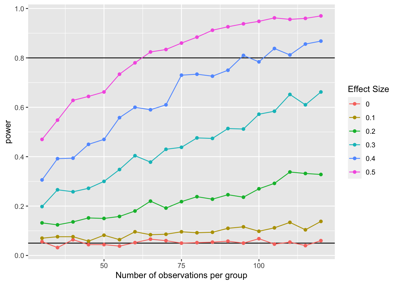
Lisa DeBruine
Professor of Psychology
Lisa DeBruine is a professor of psychology at the University of Glasgow. Her substantive research is on the social perception of faces and kinship. Her meta-science interests include team science (especially the Psychological Science Accelerator), open documentation, data simulation, web-based tools for data collection and stimulus generation, and teaching computational reproducibility.