PCA

2017-06-26 8 min read rstats

Download the Rmd notebook for this example

Putting together this page made me realise I still don’t know anything about PCA and factor analysis.

I use the psych package for SPSS-style PCA.

library(tidyverse)
library(psych)
library(viridis)

First, I’ll simulate some data with an underlying structure of three factors.

set.seed(444)  # for reproducibility; delete when running simulations

a <- rnorm(100, 0, 1)
b <- rnorm(100, 0, 1)
c <- rnorm(100, 0, 1)

df <- data.frame(
  id = seq(1,100),
  a1 = a + rnorm(100, 0, 1),
  a2 = a + rnorm(100, 0, .8),
  a3 = a + rnorm(100, 0, .6),
  a4 = -a + rnorm(100, 0, .4),
  b1 = b + rnorm(100, 0, 1),
  b2 = b + rnorm(100, 0, .8),
  b3 = b + rnorm(100, 0, .6),
  b4 = -b + rnorm(100, 0, .4),
  c1 = c + rnorm(100, 0, 1),
  c2 = c + rnorm(100, 0, .8),
  c3 = c + rnorm(100, 0, .6),
  c4 = -c + rnorm(100, 0, .4)
)

Select just the columns you want for your PCA. You can visualise their correlations with cor() and ggplot().

traits <- df %>% select(-id) 

traits %>%
  cor() %>%
  as.data.frame() %>%
  mutate(var1 = rownames(.)) %>%
  gather("var2", "value", a1:c4) %>%
  mutate(var1 = factor(var1), var1 = factor(var1, levels = rev(levels(var1)))) %>%
  ggplot(aes(var2, var1, fill=value)) +
  geom_tile() +
  scale_x_discrete(position = "top") +
  xlab("") + ylab("") +
  scale_fill_viridis(limits=c(-1, 1))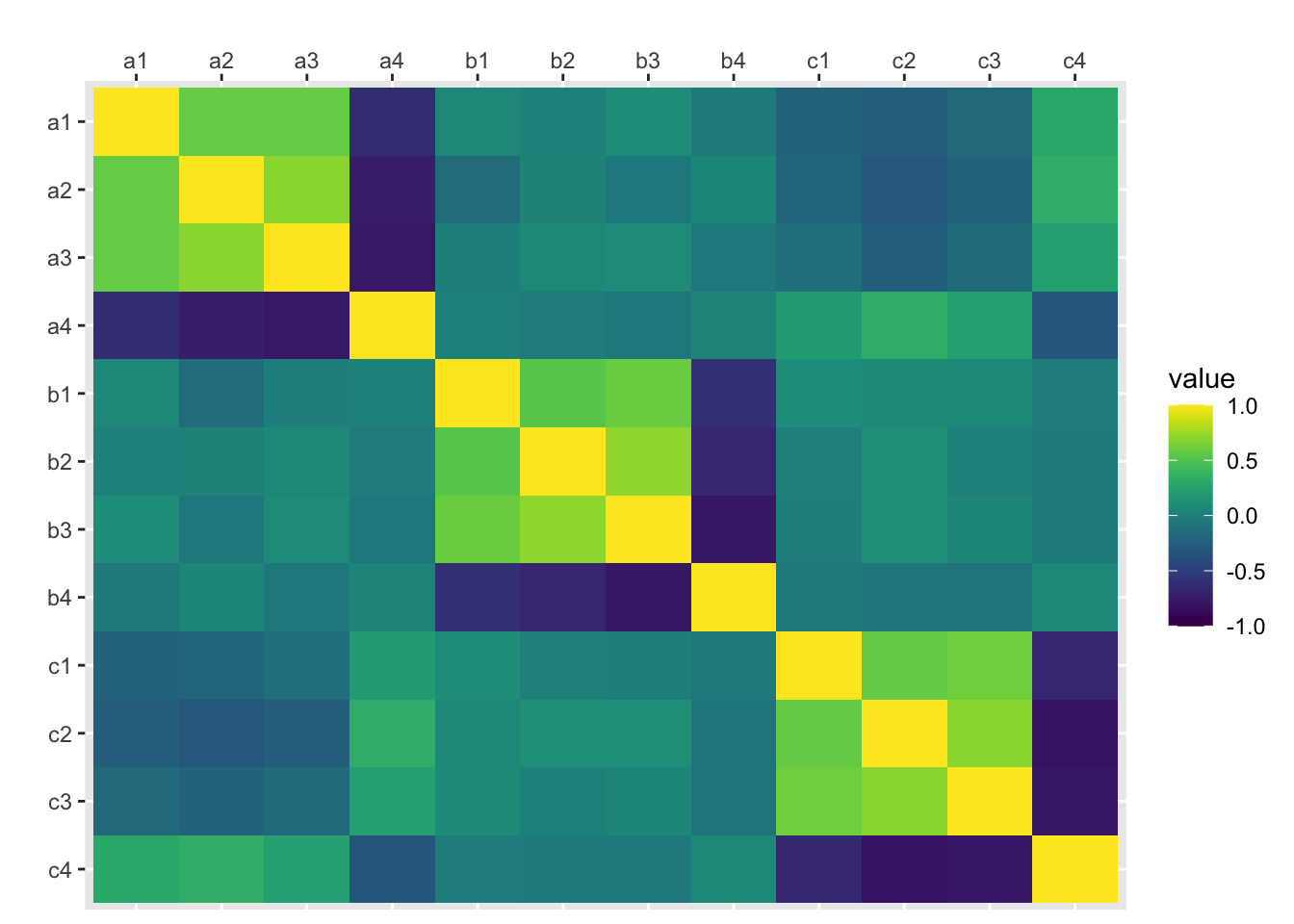

Determine the number of factors to extract. Here I use the SPSS-style default criterion of Eigenvalues > 1

ev <- eigen(cor(traits));
nfactors <- length(ev$values[ev$values > 1]);
nfactors

## [1] 3

Principal components analysis (SPSS-style)

principal(rotation = “none”)

traits.principal <- principal(traits, nfactors=nfactors, rotate="none", scores=TRUE)
traits.principal

## Principal Components Analysis
## Call: principal(r = traits, nfactors = nfactors, rotate = "none", scores = TRUE)
## Standardized loadings (pattern matrix) based upon correlation matrix
##      PC1   PC2   PC3   h2   u2 com
## a1 -0.63  0.24  0.42 0.63 0.37 2.1
## a2 -0.72  0.12  0.50 0.77 0.23 1.8
## a3 -0.65  0.26  0.55 0.79 0.21 2.3
## a4  0.73 -0.23 -0.49 0.83 0.17 2.0
## b1  0.14  0.75 -0.19 0.62 0.38 1.2
## b2  0.09  0.83 -0.16 0.71 0.29 1.1
## b3  0.10  0.89 -0.16 0.83 0.17 1.1
## b4 -0.12 -0.88  0.15 0.81 0.19 1.1
## c1  0.64  0.04  0.50 0.66 0.34 1.9
## c2  0.77  0.10  0.42 0.78 0.22 1.6
## c3  0.70  0.08  0.54 0.79 0.21 1.9
## c4 -0.80 -0.04 -0.49 0.88 0.12 1.7
## 
##                        PC1  PC2  PC3
## SS loadings           4.05 3.02 2.03
## Proportion Var        0.34 0.25 0.17
## Cumulative Var        0.34 0.59 0.76
## Proportion Explained  0.45 0.33 0.22
## Cumulative Proportion 0.45 0.78 1.00
## 
## Mean item complexity =  1.6
## Test of the hypothesis that 3 components are sufficient.
## 
## The root mean square of the residuals (RMSR) is  0.05 
##  with the empirical chi square  33.59  with prob <  0.44 
## 
## Fit based upon off diagonal values = 0.98

scores.principal <- traits.principal$scores

cor(scores.principal, traits) %>%
  as.data.frame() %>%
  mutate(var1 = rownames(.)) %>%
  gather("var2", "value", a1:c4) %>%
  mutate(var1 = factor(var1), var1 = factor(var1, levels = rev(levels(var1)))) %>%
  ggplot(aes(var2, var1, fill=value)) +
  geom_tile() +
  scale_x_discrete(position = "top") +
  xlab("") + ylab("") +
  scale_fill_viridis(limits=c(-1, 1))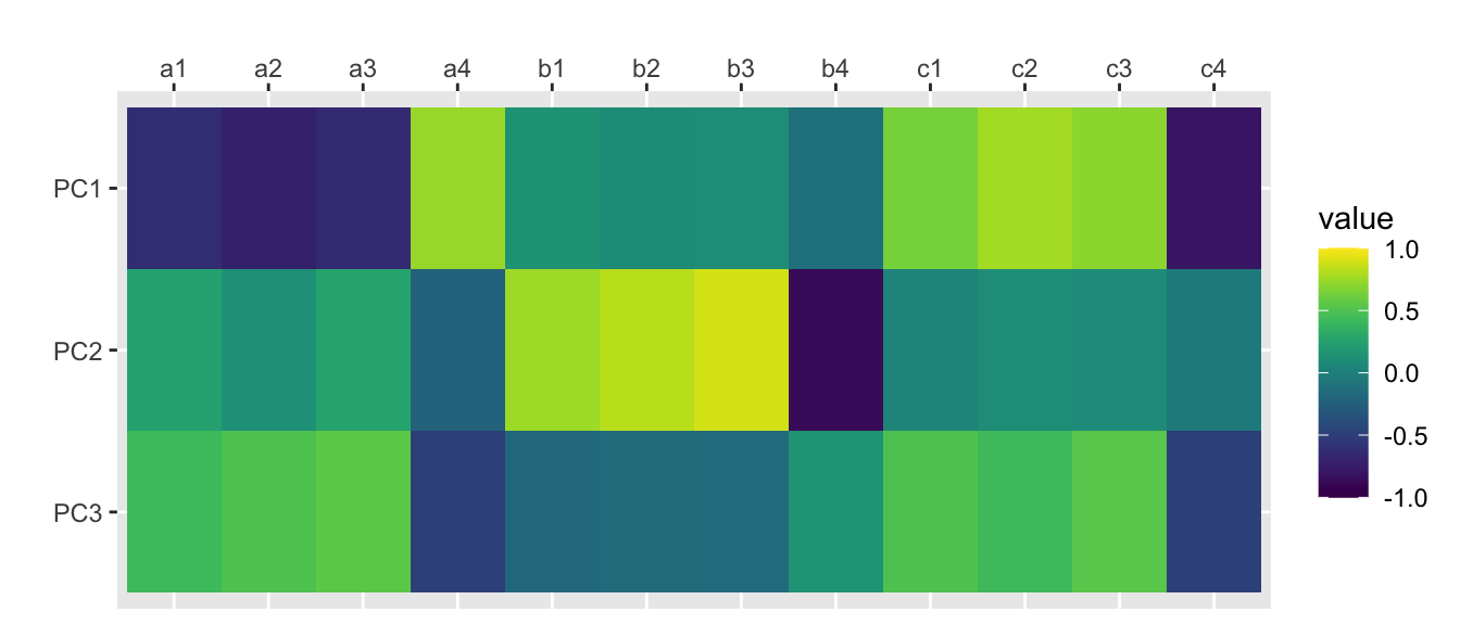

principal(rotation = “varimax”)

traits.varimax <- principal(traits, nfactors=nfactors, rotate="varimax", scores=TRUE)
traits.varimax

## Principal Components Analysis
## Call: principal(r = traits, nfactors = nfactors, rotate = "varimax", 
##     scores = TRUE)
## Standardized loadings (pattern matrix) based upon correlation matrix
##      RC1   RC3   RC2   h2   u2 com
## a1 -0.15  0.78  0.06 0.63 0.37 1.1
## a2 -0.16  0.86 -0.09 0.77 0.23 1.1
## a3 -0.07  0.89  0.05 0.79 0.21 1.0
## a4  0.17 -0.90 -0.02 0.83 0.17 1.1
## b1  0.03 -0.05  0.79 0.62 0.38 1.0
## b2  0.02  0.03  0.84 0.71 0.29 1.0
## b3  0.03  0.05  0.91 0.83 0.17 1.0
## b4 -0.05 -0.03 -0.90 0.81 0.19 1.0
## c1  0.81 -0.08  0.00 0.66 0.34 1.0
## c2  0.85 -0.21  0.09 0.78 0.22 1.1
## c3  0.88 -0.09  0.04 0.79 0.21 1.0
## c4 -0.92  0.20 -0.02 0.88 0.12 1.1
## 
##                        RC1  RC3  RC2
## SS loadings           3.09 3.03 2.98
## Proportion Var        0.26 0.25 0.25
## Cumulative Var        0.26 0.51 0.76
## Proportion Explained  0.34 0.33 0.33
## Cumulative Proportion 0.34 0.67 1.00
## 
## Mean item complexity =  1
## Test of the hypothesis that 3 components are sufficient.
## 
## The root mean square of the residuals (RMSR) is  0.05 
##  with the empirical chi square  33.59  with prob <  0.44 
## 
## Fit based upon off diagonal values = 0.98

scores.varimax <- traits.varimax$scores

cor(scores.varimax, traits) %>%
  as.data.frame() %>%
  mutate(var1 = rownames(.)) %>%
  gather("var2", "value", a1:c4) %>%
  mutate(var1 = factor(var1), var1 = factor(var1, levels = rev(levels(var1)))) %>%
  ggplot(aes(var2, var1, fill=value)) +
  geom_tile() +
  scale_x_discrete(position = "top") +
  xlab("") + ylab("") +
  scale_fill_viridis(limits=c(-1, 1))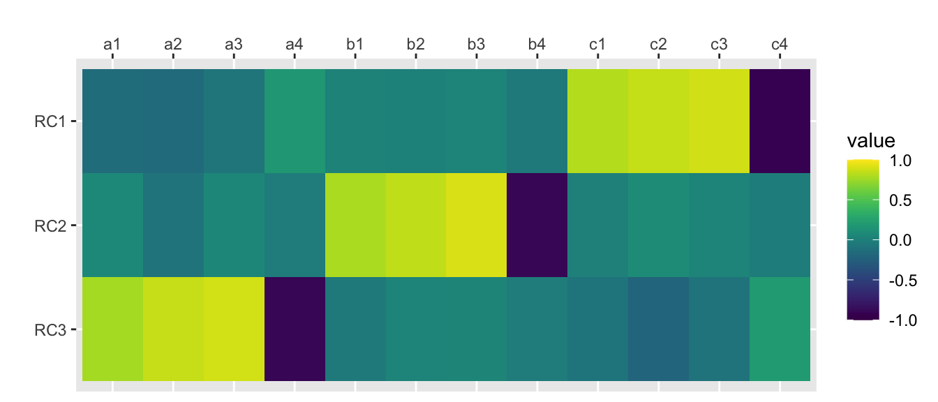

Here are some other functions for PCA/Factor Analysis

princomp()

traits.princomp <- princomp(traits)
traits.princomp$loadings[,1:nfactors]

##         Comp.1       Comp.2      Comp.3
## a1  0.33006521  0.181709692  0.45906811
## a2  0.29151833  0.067518916  0.38086462
## a3  0.23950762  0.132057875  0.38289101
## a4 -0.25823681 -0.112938603 -0.32926216
## b1 -0.10631062  0.507810878 -0.12639281
## b2 -0.07370167  0.500188081 -0.09771759
## b3 -0.06894907  0.491029731 -0.08032005
## b4  0.07460353 -0.426344256  0.07374535
## c1 -0.44100481 -0.021914387  0.38825383
## c2 -0.42646359  0.010511567  0.23488306
## c3 -0.35757417 -0.001802824  0.29574993
## c4  0.38827130  0.026358392 -0.24163371

scores.princomp <- traits.princomp$scores[,1:nfactors]

cor(scores.princomp, traits) %>%
  as.data.frame() %>%
  mutate(var1 = rownames(.)) %>%
  gather("var2", "value", a1:c4) %>%
  mutate(var1 = factor(var1), var1 = factor(var1, levels = rev(levels(var1)))) %>%
  ggplot(aes(var2, var1, fill=value)) +
  geom_tile() +
  scale_x_discrete(position = "top") +
  xlab("") + ylab("") +
  scale_fill_viridis(limits=c(-1, 1))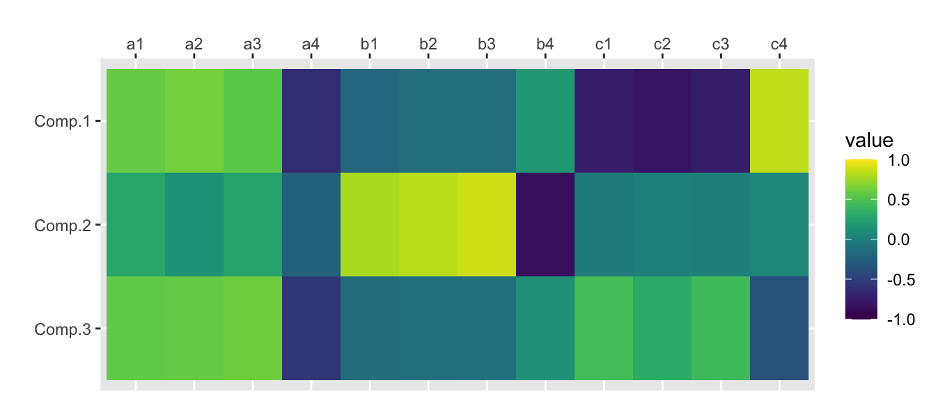

factanal(rotation = “none”)

traits.fa <- factanal(traits, nfactors, rotation="none", scores="regression")
print(traits.fa, digits=2, cutoff=0, sort=FALSE)

## 
## Call:
## factanal(x = traits, factors = nfactors, scores = "regression",     rotation = "none")
## 
## Uniquenesses:
##   a1   a2   a3   a4   b1   b2   b3   b4   c1   c2   c3   c4 
## 0.52 0.32 0.26 0.18 0.53 0.40 0.18 0.23 0.50 0.27 0.32 0.08 
## 
## Loadings:
##    Factor1 Factor2 Factor3
## a1 -0.46    0.26    0.45  
## a2 -0.55    0.17    0.60  
## a3 -0.47    0.32    0.64  
## a4  0.57   -0.30   -0.64  
## b1  0.09    0.63   -0.25  
## b2  0.07    0.74   -0.21  
## b3  0.08    0.87   -0.24  
## b4 -0.10   -0.84    0.24  
## c1  0.66    0.03    0.25  
## c2  0.83    0.09    0.19  
## c3  0.77    0.08    0.29  
## c4 -0.92   -0.05   -0.28  
## 
##                Factor1 Factor2 Factor3
## SS loadings       3.65    2.71    1.86
## Proportion Var    0.30    0.23    0.16
## Cumulative Var    0.30    0.53    0.68
## 
## Test of the hypothesis that 3 factors are sufficient.
## The chi square statistic is 22.21 on 33 degrees of freedom.
## The p-value is 0.923

scores.fa <- traits.fa$scores

cor(scores.fa, traits) %>%
  as.data.frame() %>%
  mutate(var1 = rownames(.)) %>%
  gather("var2", "value", a1:c4) %>%
  mutate(var1 = factor(var1), var1 = factor(var1, levels = rev(levels(var1)))) %>%
  ggplot(aes(var2, var1, fill=value)) +
  geom_tile() +
  scale_x_discrete(position = "top") +
  xlab("") + ylab("") +
  scale_fill_viridis(limits=c(-1, 1))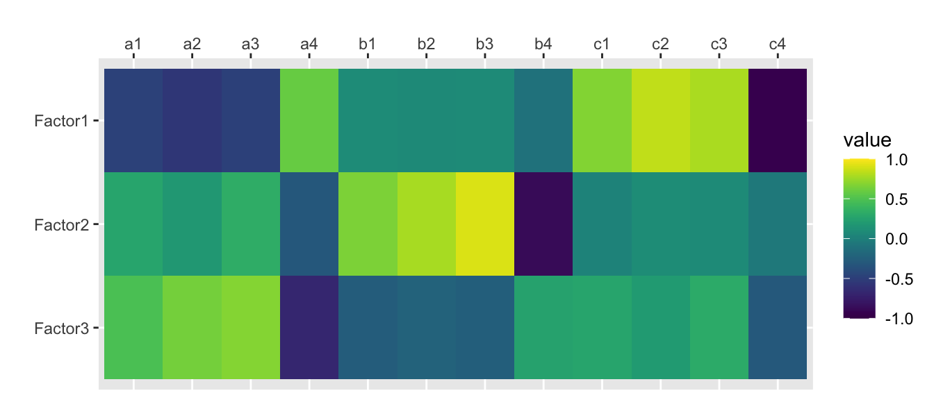

factanal(rotation = “varimax”)

traits.fa.vm <- factanal(traits, nfactors, rotation="varimax", scores="regression")
print(traits.fa.vm, digits=2, cutoff=0, sort=FALSE)

## 
## Call:
## factanal(x = traits, factors = nfactors, scores = "regression",     rotation = "varimax")
## 
## Uniquenesses:
##   a1   a2   a3   a4   b1   b2   b3   b4   c1   c2   c3   c4 
## 0.52 0.32 0.26 0.18 0.53 0.40 0.18 0.23 0.50 0.27 0.32 0.08 
## 
## Loadings:
##    Factor1 Factor2 Factor3
## a1 -0.16    0.67    0.06  
## a2 -0.18    0.80   -0.08  
## a3 -0.08    0.85    0.05  
## a4  0.17   -0.89   -0.03  
## b1  0.02   -0.04    0.68  
## b2  0.03    0.04    0.77  
## b3  0.04    0.05    0.91  
## b4 -0.05   -0.03   -0.87  
## c1  0.70   -0.10    0.00  
## c2  0.82   -0.21    0.09  
## c3  0.82   -0.11    0.04  
## c4 -0.94    0.19   -0.02  
## 
##                Factor1 Factor2 Factor3
## SS loadings       2.82    2.73    2.67
## Proportion Var    0.23    0.23    0.22
## Cumulative Var    0.23    0.46    0.68
## 
## Test of the hypothesis that 3 factors are sufficient.
## The chi square statistic is 22.21 on 33 degrees of freedom.
## The p-value is 0.923

scores.fa.vm <- traits.fa.vm$scores

cor(scores.fa.vm, traits) %>%
  as.data.frame() %>%
  mutate(var1 = rownames(.)) %>%
  gather("var2", "value", a1:c4) %>%
  mutate(var1 = factor(var1), var1 = factor(var1, levels = rev(levels(var1)))) %>%
  ggplot(aes(var2, var1, fill=value)) +
  geom_tile() +
  scale_x_discrete(position = "top") +
  xlab("") + ylab("") +
  scale_fill_viridis(limits=c(-1, 1))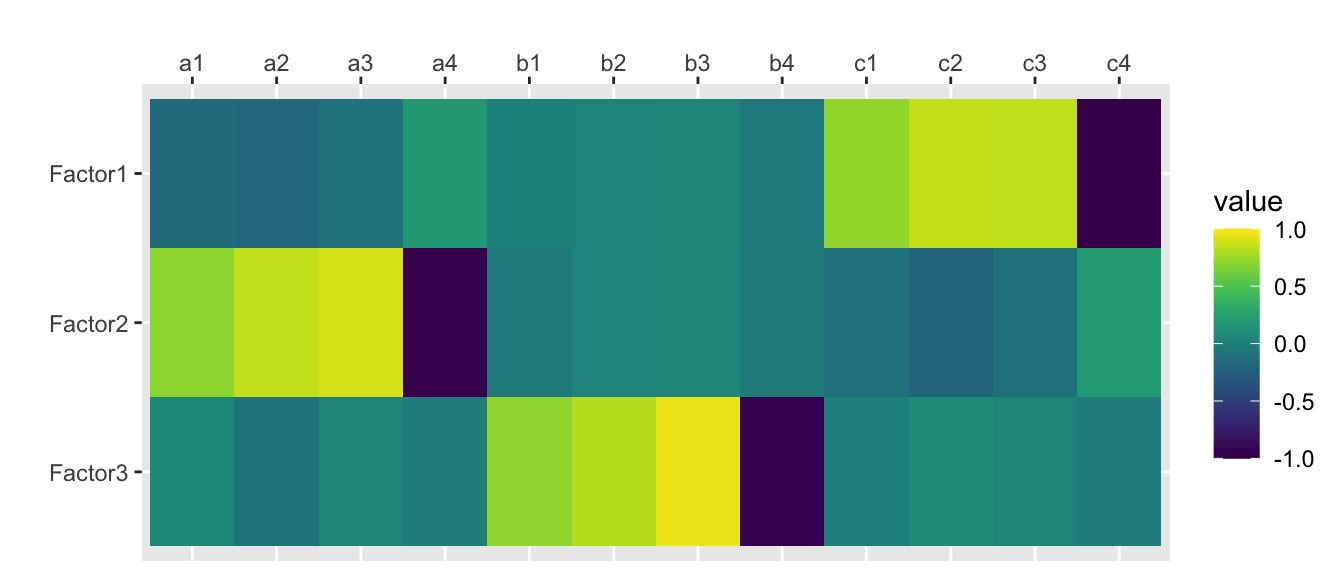

How do they compare?

Here, I’ll plot the absolute value of all the correlations (since the sign on factors/PCs is arbitrary).

The functions principal(rotation = “varimax”) and factanal(rotation = “varimax”) are nearly (but not perfectly) identical.

scores.fa <- traits.fa$scores
colnames(scores.principal) <- c("principal() 1", "principal() 2", "principal() 3")
colnames(scores.varimax) <- c("principal(vm) 1", "principal(vm) 2", "principal(vm) 3")
colnames(scores.princomp) <- c("princomp() 1", "princomp() 2", "princomp() 3")
colnames(scores.fa) <- c("factanal() 1", "factanal() 2", "factanal() 3")
colnames(scores.fa.vm) <- c("factanal(vm) 1", "factanal(vm) 2", "factanal(vm) 3")

cbind(
  scores.princomp,
  scores.principal,
  scores.fa,
  scores.varimax,
  scores.fa.vm
) %>% 
  cor() %>%
  as.data.frame() %>%
  mutate(var1 = rownames(.)) %>%
  gather("var2", "value", 1:15) %>%
  mutate(var1 = factor(var1), var1 = factor(var1, levels = rev(levels(var1)))) %>%
  mutate(value = abs(value)) %>%
  ggplot(aes(var2, var1, fill=value)) +
  geom_tile() +
  scale_x_discrete(position = "top") +
  xlab("") + ylab("") +
  scale_fill_viridis(limits=c(0, 1)) +
  geom_hline(yintercept = 3.5, color="white") +
  geom_hline(yintercept = 6.5, color="white") +
  geom_hline(yintercept = 9.5, color="white") +
  geom_hline(yintercept = 12.5, color="white") +
  geom_vline(xintercept = 3.5, color="white") +
  geom_vline(xintercept = 6.5, color="white") +
  geom_vline(xintercept = 9.5, color="white") +
  geom_vline(xintercept = 12.5, color="white") +
  theme(axis.text.x=element_text(angle=90,hjust=1))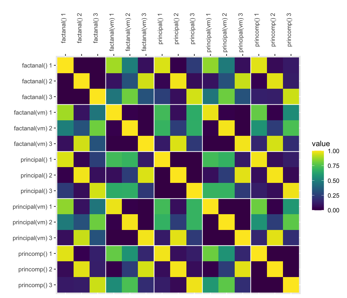

R pca princomp psych factanal

Lisa DeBruine

Professor of Psychology

Lisa DeBruine is a professor of psychology at the University of Glasgow. Her substantive research is on the social perception of faces and kinship. Her meta-science interests include team science (especially the Psychological Science Accelerator), open documentation, data simulation, web-based tools for data collection and stimulus generation, and teaching computational reproducibility.

PCA