sample()
First, let’s make a data frame with two variables, a and b that are both sampled from a normal distribution with a mean of 0 and SD of 1. The variablle n will be how many samples we’ll take (100). Then we can run a t-test to see if they are different.
library(tidyverse)## ── Attaching packages ────────────────────── tidyverse 1.3.0 ──## ✓ ggplot2 3.3.2 ✓ purrr 0.3.4
## ✓ tibble 3.0.3 ✓ dplyr 1.0.2
## ✓ tidyr 1.1.1 ✓ stringr 1.4.0
## ✓ readr 1.3.1 ✓ forcats 0.5.0## ── Conflicts ───────────────────────── tidyverse_conflicts() ──
## x dplyr::filter() masks stats::filter()
## x dplyr::lag() masks stats::lag()n = 100
data <- data.frame(
a = rnorm(n, 0, 1),
b = rnorm(n, 0, 1)
)
t <- t.test(data$a,data$b)
t$p.value## [1] 0.1527518Now let’s repeat that procedure 1000 times. The easiest way to do that is to make a function that returns the information you want.
tPower <- function() {
  n = 100

  data <- data.frame(
    a = rnorm(n, 0, 1),
    b = rnorm(n, 0, 1)
  )

  t <- t.test(data$a,data$b)

  return(t$p.value)
}

tPower()
## [1] 0.7583175mySample <- data.frame(
p = replicate(10000, tPower())
)
mySample %>%
ggplot(aes(p)) +
geom_histogram(bins = 20, boundary = 0)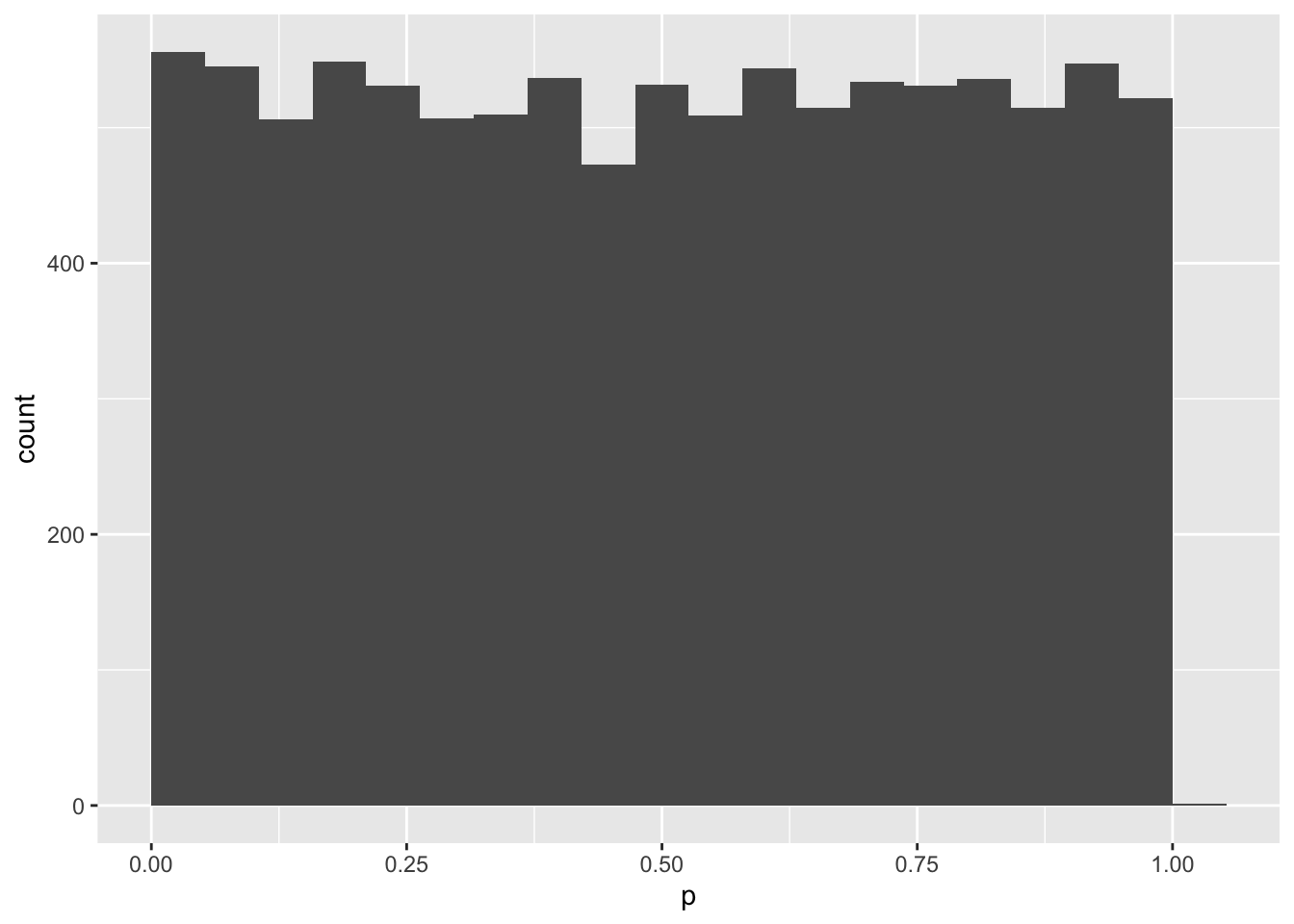
mean(mySample$p < .05)## [1] 0.0528What if you induced a small effect of 0.2 SD?
tPower2 <- function() {
  n = 100

  data <- data.frame(
    a = rnorm(n, 0, 1),
    b = rnorm(n, 0.2, 1)
  )

  t <- t.test(data$a,data$b)

  return(t$p.value)
}

tPower2()
## [1] 0.9142489mySample2 <- data.frame(
p = replicate(10000, tPower2())
)
mySample2 %>%
ggplot(aes(p)) +
geom_histogram(bins = 20, boundary = 0)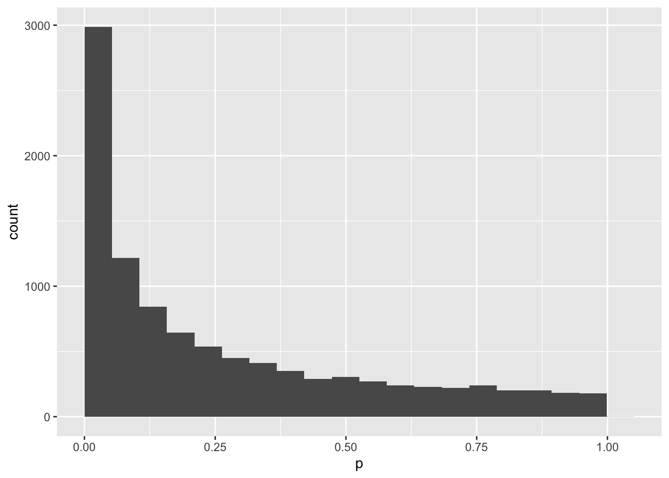
mean(mySample2$p < .05)## [1] 0.2929Hmm, you only get a p-value less than .05 30% of the time. That means that your study would only have 30% power to detect an effect this big with 100 subjects. Let’s make a new function to give you the p-value of a study with any number of subjects (you put the N inside the parentheses of the function).
tPowerN <- function(n) {

  data <- data.frame(
    a = rnorm(n, 0, 1),
    b = rnorm(n, 0.2, 1)
  )

  t <- t.test(data$a,data$b)

  return(t$p.value)
}

tPowerN(200)
## [1] 0.2969539mySampleN <- data.frame(
p200 = replicate(10000, tPowerN(200))
)
mySampleN %>%
ggplot(aes(p200)) +
geom_histogram(bins = 20, boundary = 0)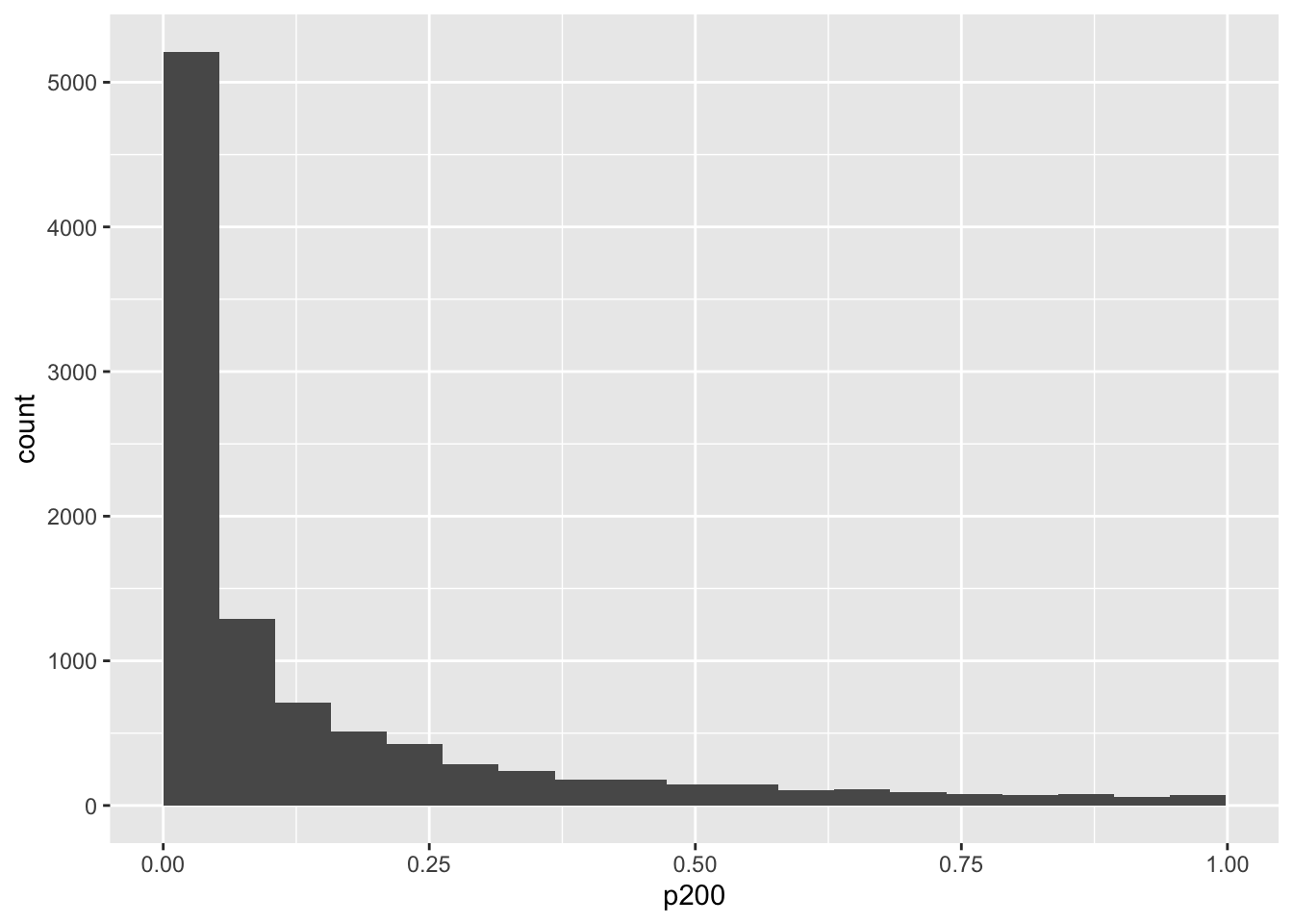
mean(mySampleN$p200 < .05)## [1] 0.5137nlist <- seq(200, 1000, by = 100)
remove(mySampleN)
for (n in nlist) {
temp <- data.frame(
n = n,
p = replicate(1000, tPowerN(n))
)
if (exists("mySampleN")) {
mySampleN <- rbind(mySampleN, temp)
} else {
mySampleN <- temp
}
remove(temp)
print(n)
}## [1] 200
## [1] 300
## [1] 400
## [1] 500
## [1] 600
## [1] 700
## [1] 800
## [1] 900
## [1] 1000mySampleN %>%
ggplot(aes(p)) +
geom_histogram(bins = 20, boundary = 0) +
facet_wrap(~n, nrow = 3)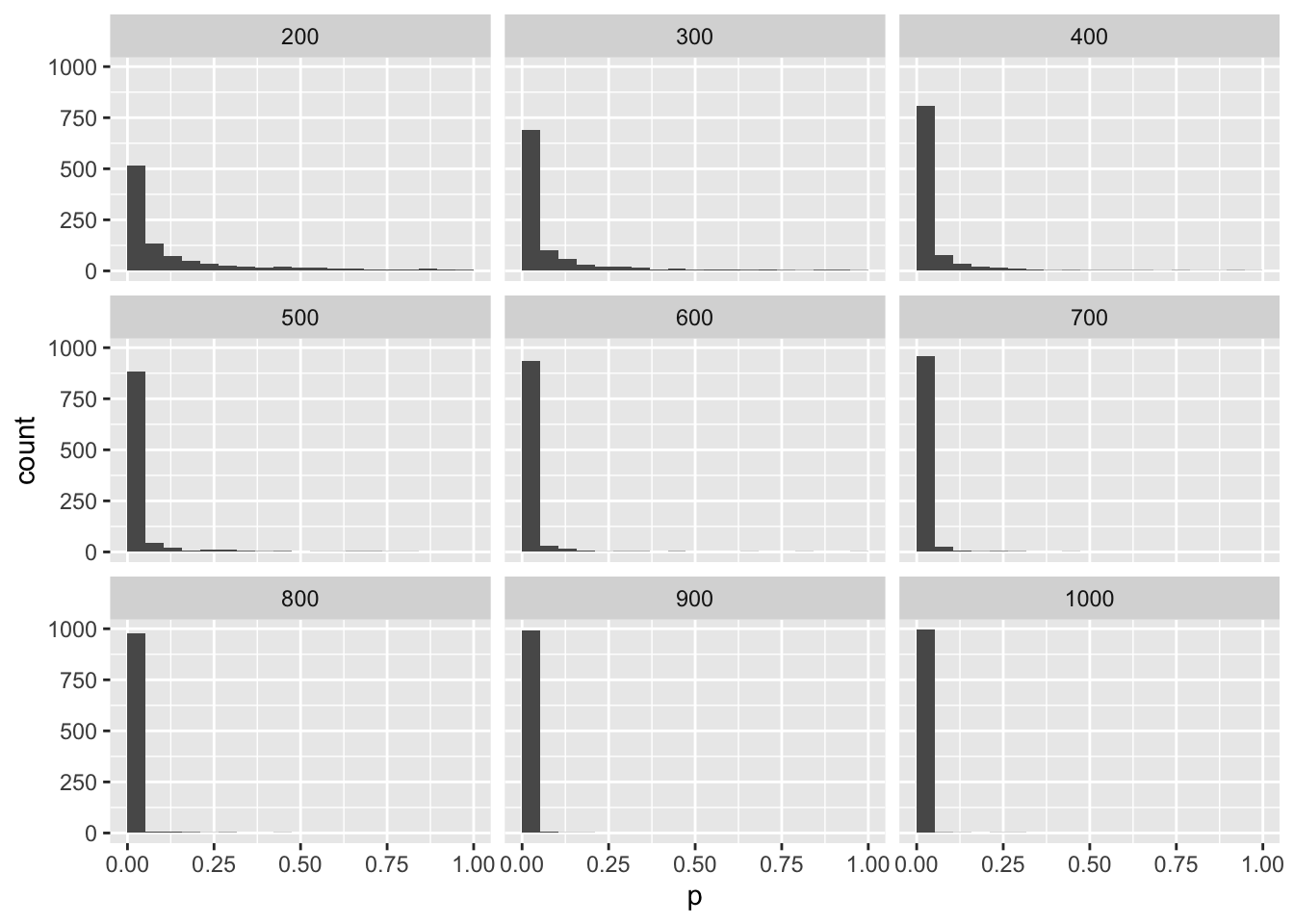
Lisa DeBruine
Professor of Psychology
Lisa DeBruine is a professor of psychology at the University of Glasgow. Her substantive research is on the social perception of faces and kinship. Her meta-science interests include team science (especially the Psychological Science Accelerator), open documentation, data simulation, web-based tools for data collection and stimulus generation, and teaching computational reproducibility.