Contrasts other than treatment coding for factors with more than two levels have always confused me. I try to design all my own studies to never have more than two levels per categorical factor, but students in my data skills class are always trying to analyse data with three-level categories (or worse).
I thought it was just me, but some recent Twitter discussion showed me I’m not alone. There’s a serious jingle-jangle problem with contrasts. Here are some of the explainers that I found useful (thanks to everyone who recommended them).
- Contrasts in R by Marissa Barlaz
- Coding categorical predictor variables in factorial designs by Dale Barr
- Contrast Coding in Multiple Regression Analysis by Matthew Davis
- R Library Contrast Coding Systems for categorical variables by UCLA Statistical Consulting
- Rosetta store: Contrasts by GAMLj
- Coding Schemes for Categorical Variables by Phillip Alday
- Experimental personality designs: analyzing categorical by continuous variable interactions by West, Aiken & Krull
Terminology
Contrasts often have multiple names. The names I’m using try to maintain the relationship with the base R function, apart from anova coding, which was suggested by Dale Barr after I got frustrated that people use so many different labels for that (extremely useful) coding and each of the terms used is also used to refer to totally different codings by others.
| My name | Other names | R function | faux function |
|---|---|---|---|
| Treatment | Treatment (2), Dummy (1, 4, 6), Simple (5) | contr.treatment |
contr_code_treatment |
| Anova | Deviation (2), Contrast (1), Simple (4) | contr.treatment - 1/k |
contr_code_anova |
| Sum | Sum (1, 2, 6), Effects (3), Deviation (4, 5), Unweighted Effects (7) | contr.sum |
contr_code_sum |
| Difference | Contrast (3), Forward/Backward (4), Repeated (5) | MASS::contr.sdif |
contr_code_difference |
| Helmert | Reverse Helmert (1, 4), Difference (5), Contrast (7) | contr.helmert / (column_i+1) |
contr_code_helmert |
| Polynomial | Polynomial (5), Orthogonal Polynomial (4), Trend (3) | contr.poly |
contr_code_poly |
Faux Contrast Functions
These functions are under development
First, we’ll set up a simple experimental design and analyse it with
lm(). I set empirical = TRUE to make
interpreting the estimates easier.
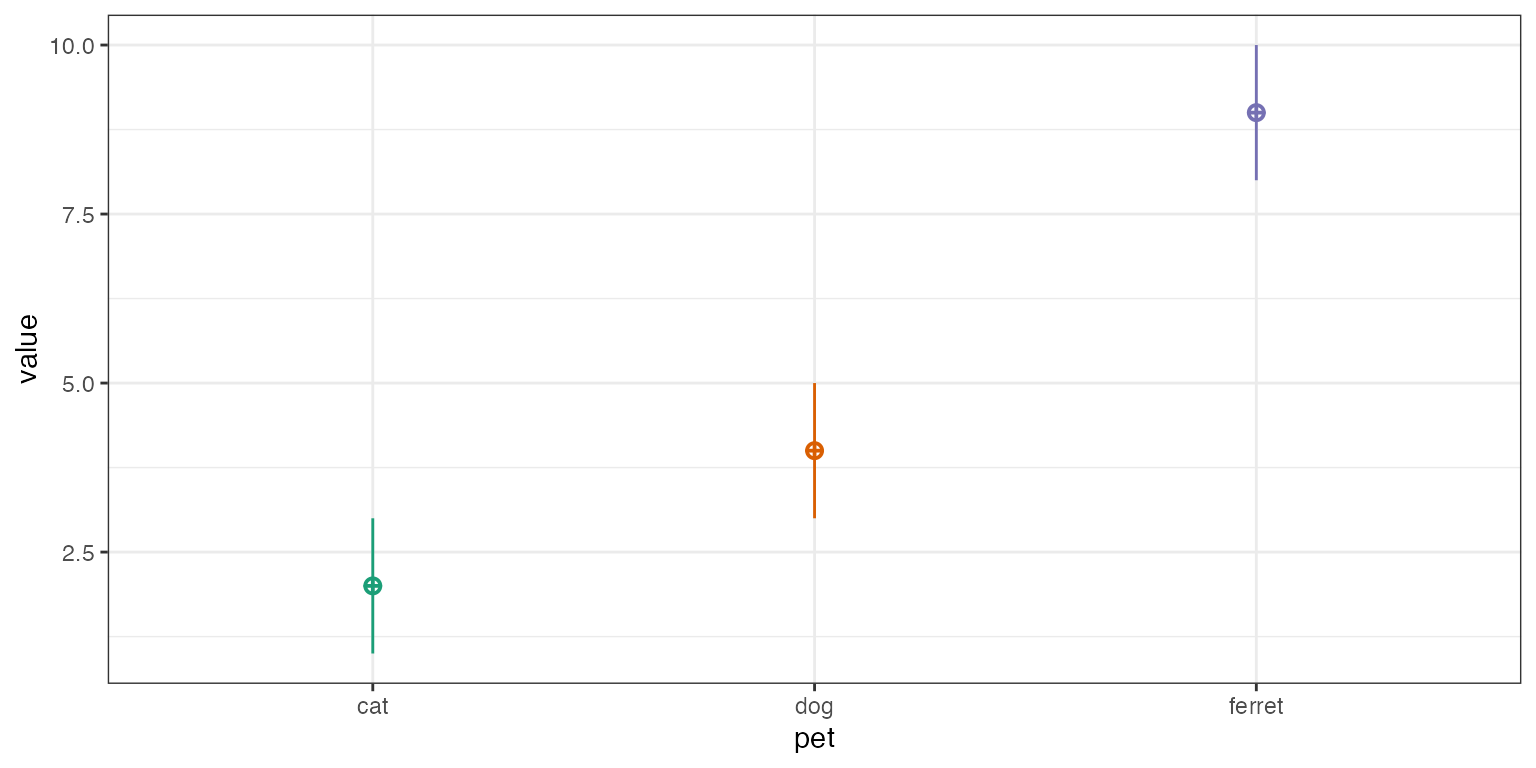
df <- sim_design(between = list(pet = c("cat", "dog", "ferret")),
                 n = c(50), mu = c(2, 4, 9), empirical = TRUE)
Notice that the default contrast is treatment coding, with “cat” as
the baseline condition. The estimate for the intercept is the mean value
for cats
(),
while the term petdog is the mean value for dogs minus cats
(),
and the term petferret is the mean value for ferrets minus
cats
().
| Contrasts | lm(y ~ pet, df) | ||||||||||||||||||||||||||||||||
|---|---|---|---|---|---|---|---|---|---|---|---|---|---|---|---|---|---|---|---|---|---|---|---|---|---|---|---|---|---|---|---|---|---|
|
|
In all the subsequent examples, try putting into words what the estimates for the intercept and terms mean in relation to the mean values for each group in the data.
Treatment coding (also called dummy coding) sets the mean of the
reference group as the intercept. It is straightforward to interpret,
especially when your factors have an obvious default or baseline value.
This is the same type of coding as the default for factors shown above
(unless you change your default using options()), but with
clearer term labels.
df$pet <- contr_code_treatment(df$pet)| Contrasts | lm(y ~ pet, df) | ||||||||||||||||||||||||||||||||
|---|---|---|---|---|---|---|---|---|---|---|---|---|---|---|---|---|---|---|---|---|---|---|---|---|---|---|---|---|---|---|---|---|---|
|
|
Each contrast compares one level with the reference level, which
defaults to the first level, but you can set with the base
argument. Now the intercept estimates the mean value for dogs
().
df$pet <- contr_code_treatment(df$pet, base = "dog")| Contrasts | lm(y ~ pet, df) | ||||||||||||||||||||||||||||||||
|---|---|---|---|---|---|---|---|---|---|---|---|---|---|---|---|---|---|---|---|---|---|---|---|---|---|---|---|---|---|---|---|---|---|
|
|
Set the reference level to the third level (“ferret”).
df$pet <- contr_code_treatment(df$pet, base = 3)| Contrasts | lm(y ~ pet, df) | ||||||||||||||||||||||||||||||||
|---|---|---|---|---|---|---|---|---|---|---|---|---|---|---|---|---|---|---|---|---|---|---|---|---|---|---|---|---|---|---|---|---|---|
|
|
Anova coding is identical to treatment coding, but sets the grand mean as the intercept. Each contrast compares one level with a reference level. This gives us values that are relatively easy to interpret and map onto ANOVA values.
Below is anova coding with the first level (“cat”) as the default
base. Now the intercept is the grand mean, which is the mean of the
three group means
().
Notice that this is different from the mean value of y in our dataset
(5, since the number of pets in each group is unbalanced. The term
pet_dog-cat is the mean value for dogs minus cats
()
and the term pet_ferret-cat is the mean value for ferrets
minus cats
().
df$pet <- contr_code_anova(df$pet)| Contrasts | lm(y ~ pet, df) | ||||||||||||||||||||||||||||||||
|---|---|---|---|---|---|---|---|---|---|---|---|---|---|---|---|---|---|---|---|---|---|---|---|---|---|---|---|---|---|---|---|---|---|
|
|
Anova coding with “dog” as the base. How does the interpretation of the terms change?
df$pet <- contr_code_anova(df$pet, base = "dog")| Contrasts | lm(y ~ pet, df) | ||||||||||||||||||||||||||||||||
|---|---|---|---|---|---|---|---|---|---|---|---|---|---|---|---|---|---|---|---|---|---|---|---|---|---|---|---|---|---|---|---|---|---|
|
|
Anova coding with the third level (“ferret”) as the base.
df$pet <- contr_code_anova(df$pet, base = 3)| Contrasts | lm(y ~ pet, df) | ||||||||||||||||||||||||||||||||
|---|---|---|---|---|---|---|---|---|---|---|---|---|---|---|---|---|---|---|---|---|---|---|---|---|---|---|---|---|---|---|---|---|---|
|
|
Sum coding also sets the grand mean as the intercept. Each contrast
compares one level with the grand mean. Therefore, the estimate for
pet_cat-intercept is the difference between the mean value
for cats and the grand mean
().
df$pet <- contr_code_sum(df$pet)| Contrasts | lm(y ~ pet, df) | ||||||||||||||||||||||||||||||||
|---|---|---|---|---|---|---|---|---|---|---|---|---|---|---|---|---|---|---|---|---|---|---|---|---|---|---|---|---|---|---|---|---|---|
|
|
You can’t compare all levels with the grand mean, and have to omit
one level. This is the last level by default, but you can change it with
the omit argument.
df$pet <- contr_code_sum(df$pet, omit = "dog")| Contrasts | lm(y ~ pet, df) | ||||||||||||||||||||||||||||||||
|---|---|---|---|---|---|---|---|---|---|---|---|---|---|---|---|---|---|---|---|---|---|---|---|---|---|---|---|---|---|---|---|---|---|
|
|
Omit the first level (“cat”).
df$pet <- contr_code_sum(df$pet, omit = 1)| Contrasts | lm(y ~ pet, df) | ||||||||||||||||||||||||||||||||
|---|---|---|---|---|---|---|---|---|---|---|---|---|---|---|---|---|---|---|---|---|---|---|---|---|---|---|---|---|---|---|---|---|---|
|
|
A slightly different form of contrast coding is difference coding, also called forward, backward, or successive differences coding. It compares each level to the previous one, rather than to a baseline level.
df$pet <- contr_code_difference(df$pet)| Contrasts | lm(y ~ pet, df) | ||||||||||||||||||||||||||||||||
|---|---|---|---|---|---|---|---|---|---|---|---|---|---|---|---|---|---|---|---|---|---|---|---|---|---|---|---|---|---|---|---|---|---|
|
|
If you want to change which levels are compared, you can re-order the factor levels.
df$pet <- contr_code_difference(df$pet, levels = c("ferret", "cat", "dog"))| Contrasts | lm(y ~ pet, df) | ||||||||||||||||||||||||||||||||
|---|---|---|---|---|---|---|---|---|---|---|---|---|---|---|---|---|---|---|---|---|---|---|---|---|---|---|---|---|---|---|---|---|---|
|
|
Helmert coding sets the grand mean as the intercept. Each contrast
compares one level with the mean of previous levels. This coding is
somewhat different than the results from
stats::contr.helmert() to make it easier to interpret the
estimates. Thus, pet_ferret-cat.dog is the mean value for
ferrets minus the mean value for cats and dogs averaged together
().
df$pet <- contr_code_helmert(df$pet)| Contrasts | lm(y ~ pet, df) | ||||||||||||||||||||||||||||||||
|---|---|---|---|---|---|---|---|---|---|---|---|---|---|---|---|---|---|---|---|---|---|---|---|---|---|---|---|---|---|---|---|---|---|
|
|
You can change the comparisons by reordering the levels.
df$pet <- contr_code_helmert(df$pet, levels = c("ferret", "dog", "cat"))| Contrasts | lm(y ~ pet, df) | ||||||||||||||||||||||||||||||||
|---|---|---|---|---|---|---|---|---|---|---|---|---|---|---|---|---|---|---|---|---|---|---|---|---|---|---|---|---|---|---|---|---|---|
|
|
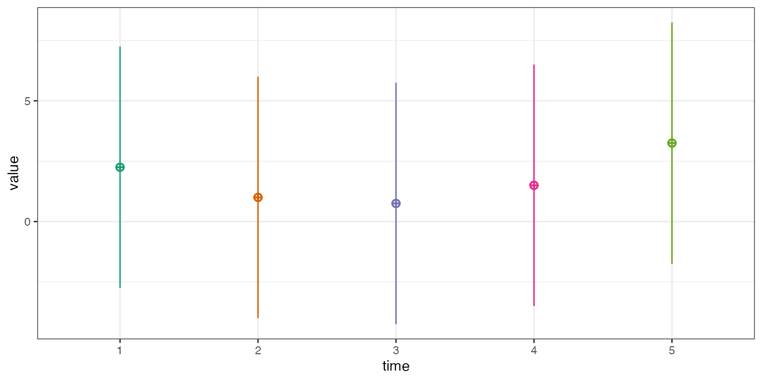
Polynomial coding is the default for ordered factors in R. We’ll set up a new data simulation with five ordered times.
df <- sim_design(list(time = 1:5),
                 mu = 1:5 * 0.25 + (1:5 - 3)^2 * 0.5,
                 sd = 5, long = TRUE)
The function contr_code_poly() uses
contr.poly() to set up the polynomial contrasts for the
linear (^1), quadratic (^2), cubic
(^3), and quartic (^4) components.
df$time <- contr_code_poly(df$time)| Contrasts | lm(y ~ pet, df) | ||||||||||||||||||||||||||||||||||||||||||||||||||||||
|---|---|---|---|---|---|---|---|---|---|---|---|---|---|---|---|---|---|---|---|---|---|---|---|---|---|---|---|---|---|---|---|---|---|---|---|---|---|---|---|---|---|---|---|---|---|---|---|---|---|---|---|---|---|---|---|
|
|
Add Contrasts
The function add_contrasts() lets you add contrasts to a
column in a data frame and also adds new columns for each contrast
(unless add_cols = FALSE). This is especially helpful if
you want to test only a subset of the contrasts.
df <- sim_design(list(time = 1:5),
                 mu = 1:5 * 0.25 + (1:5 - 3)^2 * 0.5,
                 sd = 5, long = TRUE, plot = FALSE) %>%
add_contrast("time", "poly")| term | estimate | std.error | statistic | p.value |
|---|---|---|---|---|
| (Intercept) | 1.69 | 0.239 | 7.09 | 0.000 |
time^1
|
0.78 | 0.534 | 1.46 | 0.145 |
time^2
|
2.06 | 0.534 | 3.85 | 0.000 |
You can set colnames to change the default column names
for the contrasts. This can be useful if you want to add different
codings for the same factor or if the default names are too long.
btwn <- list(condition = c("control", "experimental"))

df <- sim_design(between = btwn, n = 1, plot = FALSE) %>%
  add_contrast("condition", "treatment", colnames = "cond.tr") %>%
  add_contrast("condition", "anova", colnames = "cond.aov") %>%
  add_contrast("condition", "difference", colnames = "cond.dif") %>%
  add_contrast("condition", "sum", colnames = "cond.sum") %>%
  add_contrast("condition", "helmert", colnames = "cond.hmt") %>%
add_contrast("condition", "poly", colnames = "cond.poly")| id | condition | y | cond.tr | cond.aov | cond.dif | cond.sum | cond.hmt | cond.poly |
|---|---|---|---|---|---|---|---|---|
| S1 | control | 0.697 | 0 | -0.5 | -0.5 | 1 | -0.5 | -0.707 |
| S2 | experimental | 0.512 | 1 | 0.5 | 0.5 | -1 | 0.5 | 0.707 |
However, if a new column has a duplicate name to an existing column,
add_contrast() will automatically add a contrast suffix to
the new column.
btwn <- list(pet = c("cat", "dog", "ferret"))

df <- sim_design(between = btwn, n = 1, plot = FALSE) %>%
  add_contrast("pet", "treatment") %>%
  add_contrast("pet", "anova") %>%
  add_contrast("pet", "sum") %>%
  add_contrast("pet", "difference") %>%
  add_contrast("pet", "helmert") %>%
add_contrast("pet", "poly")| id | pet | y | pet.dog-cat | pet.ferret-cat | pet.cat-intercept | pet.dog-intercept | pet.ferret-dog | pet.ferret-cat.dog | pet^1 | pet^2 |
|---|---|---|---|---|---|---|---|---|---|---|
| S1 | cat | -0.72 | -0.5 | -0.33 | 1 | 0 | -0.33 | -0.33 | -0.71 | 0.41 |
| S2 | dog | -0.36 | 0.5 | -0.33 | 0 | 1 | -0.33 | -0.33 | 0.00 | -0.82 |
| S3 | ferret | -1.43 | 0.0 | 0.67 | -1 | -1 | 0.67 | 0.67 | 0.71 | 0.41 |
Examples
2x2 Design
Let’s use simulated data with empirical = TRUE to
explore how to interpret interactions between two 2-level factors coded
in different ways.
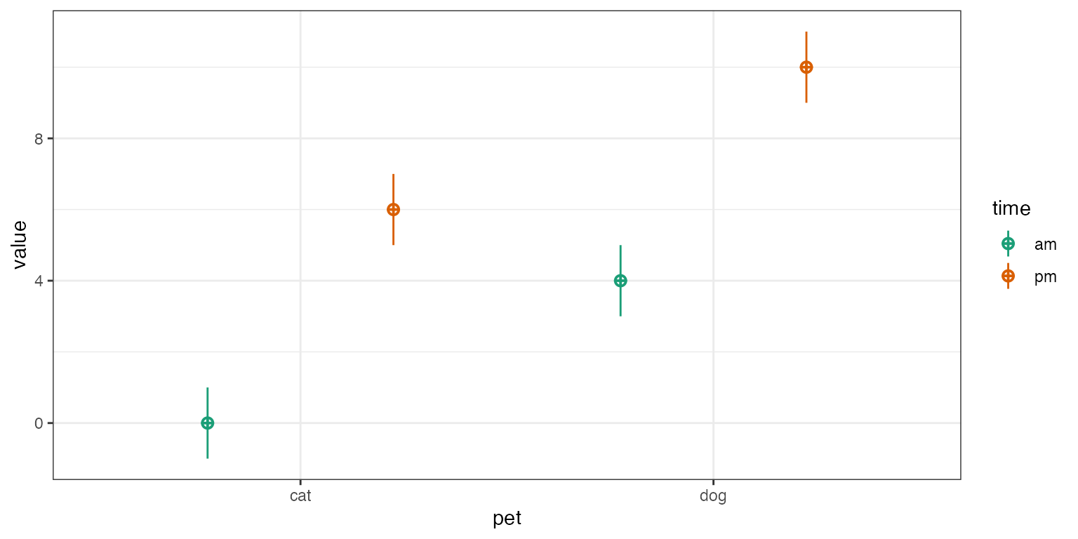
mu <- c(0, 4, 6, 10)
df <- sim_design(between = list(time = c("am", "pm"),
                                pet = c("cat", "dog")),
                 n = c(50, 60, 70, 80), mu = mu, empirical = TRUE)
The table below shows the cell and marginal means. The notation
is used to denote a mean for a specific grouping. The . is
used to indicate the mean over all groups of that factor;
Y.. is the grand mean. While you’ll usually see the
subscripts written as numbers to indicate the factor levels, we’re using
letters here so you don’t have to keep referring to the order of factors
and levels.
| cat | dog | mean | |
|---|---|---|---|
| am | |||
| pm | |||
| mean |
| term | interpretation | formula | value |
|---|---|---|---|
| intercept | cat when am | ||
| pet.dog-cat | dog minus cat, when am | ||
| time.pm-am | pm minus am, for cats | ||
| pet.dog-cat:time.pm-am | dog minus cat when pm, minus dog minus cat when am |
df %>%
  add_contrast("pet", "treatment") %>%
  add_contrast("time", "treatment") %>%
  lm(y ~ pet * time, .) %>%
broom::tidy() %>% kable() %>% kable_styling()| term | estimate | std.error | statistic | p.value |
|---|---|---|---|---|
| (Intercept) | 0 | 0.141 | 0.0 | 1 |
| pet.dog-cat | 4 | 0.191 | 20.9 | 0 |
| time.pm-am | 6 | 0.185 | 32.4 | 0 |
| pet.dog-cat:time.pm-am | 0 | 0.252 | 0.0 | 1 |
| term | interpretation | formula | value |
|---|---|---|---|
| intercept | grand mean | ||
| pet.dog-cat | mean dog minus mean cat | ||
| time.pm-am | mean pm minus mean am | ||
| pet.dog-cat:time.pm-am | dog minus cat when pm, minus dog minus cat when am |
df %>%
  add_contrast("pet", "anova") %>%
  add_contrast("time", "anova") %>%
  lm(y ~ pet * time, .) %>%
broom::tidy() %>% kable() %>% kable_styling()| term | estimate | std.error | statistic | p.value |
|---|---|---|---|---|
| (Intercept) | 5 | 0.063 | 79.4 | 0 |
| pet.dog-cat | 4 | 0.126 | 31.8 | 0 |
| time.pm-am | 6 | 0.126 | 47.6 | 0 |
| pet.dog-cat:time.pm-am | 0 | 0.252 | 0.0 | 1 |
| term | interpretation | formula | value |
|---|---|---|---|
| intercept | grand mean | ||
| pet.cat-intercept | mean cat minus grand mean | ||
| time.am-intercept | mean am minus grand mean | ||
| pet.cat-intercept:time.am-intercept | cat minus mean when am, minus cat minus mean when pm, divided by 2 |
df %>%
  add_contrast("pet", "sum") %>%
  add_contrast("time", "sum") %>%
  lm(y ~ pet * time, .) %>%
broom::tidy() %>% kable() %>% kable_styling()| term | estimate | std.error | statistic | p.value |
|---|---|---|---|---|
| (Intercept) | 5 | 0.063 | 79.4 | 0 |
| pet.cat-intercept | -2 | 0.063 | -31.8 | 0 |
| time.am-intercept | -3 | 0.063 | -47.6 | 0 |
| pet.cat-intercept:time.am-intercept | 0 | 0.063 | 0.0 | 1 |
| term | interpretation | formula | value |
|---|---|---|---|
| intercept | grand mean | ||
| pet.dog-cat | mean dog minus mean cat | ||
| time.pm-am | mean pm minus mean am | ||
| pet.dog-cat:time.pm-am | dog minus cat when pm, minus dog minus cat when am |
df %>%
  add_contrast("pet", "difference") %>%
  add_contrast("time", "difference") %>%
  lm(y ~ pet * time, .) %>%
broom::tidy() %>% kable() %>% kable_styling()| term | estimate | std.error | statistic | p.value |
|---|---|---|---|---|
| (Intercept) | 5 | 0.063 | 79.4 | 0 |
| pet.dog-cat | 4 | 0.126 | 31.8 | 0 |
| time.pm-am | 6 | 0.126 | 47.6 | 0 |
| pet.dog-cat:time.pm-am | 0 | 0.252 | 0.0 | 1 |
| term | interpretation | formula | value |
|---|---|---|---|
| intercept | grand mean | ||
| pet.dog-cat | mean dog minus mean cat | ||
| time.pm-am | mean pm minus mean am | ||
| pet.dog-cat:time.pm-am | dog minus cat when pm, minus dog minus cat when am |
df %>%
  add_contrast("pet", "helmert") %>%
  add_contrast("time", "helmert") %>%
  lm(y ~ pet * time, .) %>%
broom::tidy() %>% kable() %>% kable_styling()| term | estimate | std.error | statistic | p.value |
|---|---|---|---|---|
| (Intercept) | 5 | 0.063 | 79.4 | 0 |
| pet.dog-cat | 4 | 0.126 | 31.8 | 0 |
| time.pm-am | 6 | 0.126 | 47.6 | 0 |
| pet.dog-cat:time.pm-am | 0 | 0.252 | 0.0 | 1 |
N.B. In the case of 2-level factors, anova, difference, and Helmert coding are identical. Treatment coding differs only in the intercept.
Remember that interactions can always be described in two ways, since
(A1 - A2) - (B1 - B2) == (A1 - B1) - (A2 - B2). Therefore,
“dog minus cat when pm, minus dog minus cat when am” is the same as “pm
minus am for dogs, minus pm minus am for cats”. The way you describe it
in a paper depends on which version maps onto your hypothesis more
straightforwardly. The examples above might be written as “the
difference between dogs and cats was bigger in the evening than the
morning” or “the difference between evening and morning was bigger for
dogs than for cats”. Make sure you check the plots to make sure you are
describing the relationships in the right direction.
2x3 Design
Let’s use simulated data with empirical = TRUE to
explore how to interpret interactions between a 2-level factor and a
3-level factor coded in different ways.
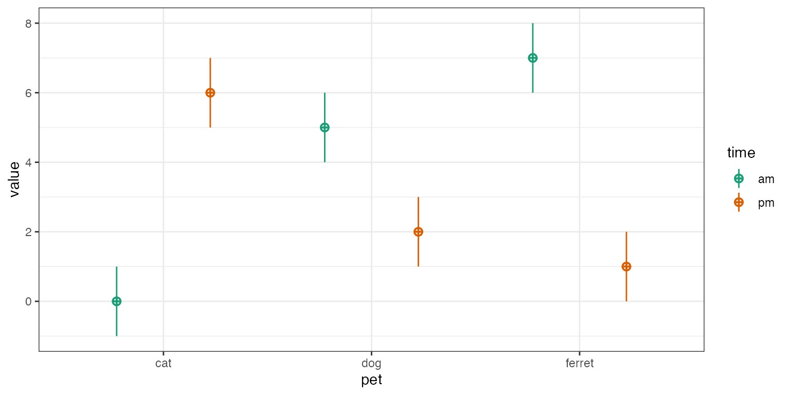
mu <- c(0, 5, 7, 6, 2, 1)
df <- sim_design(between = list(time = c("am", "pm"),
                                pet = c("cat", "dog", "ferret")),
                 n = c(50, 60, 70, 80, 90, 100), mu = mu, empirical = TRUE)
| cat | dog | ferret | mean | |
|---|---|---|---|---|
| am | ||||
| pm | ||||
| mean |
| term | interpretation | formula | value |
|---|---|---|---|
| intercept | cat when am | ||
| pet.dog-cat | dog minus cat, when am | ||
| pet.ferret-cat | ferret minus cat, when am | ||
| time.pm-am | pm minus am, for cats | ||
| pet.dog-cat:time.pm-am | dog minus cat when pm, minus dog minus cat when am | ||
| pet.ferret-cat:time.pm-am | ferret minus cat when pm, minus ferret minus cat when am |
df %>%
  add_contrast("pet", "treatment") %>%
  add_contrast("time", "treatment") %>%
  lm(y ~ pet * time, .) %>%
broom::tidy() %>% kable() %>% kable_styling()| term | estimate | std.error | statistic | p.value |
|---|---|---|---|---|
| (Intercept) | 0 | 0.141 | 0.0 | 1 |
| pet.dog-cat | 5 | 0.191 | 26.1 | 0 |
| pet.ferret-cat | 7 | 0.185 | 37.8 | 0 |
| time.pm-am | 6 | 0.180 | 33.3 | 0 |
| pet.dog-cat:time.pm-am | -9 | 0.246 | -36.7 | 0 |
| pet.ferret-cat:time.pm-am | -12 | 0.238 | -50.4 | 0 |
| term | interpretation | formula | value |
|---|---|---|---|
| intercept | grand mean | ||
| pet.dog-cat | mean dog minus mean cat | ||
| pet.ferret-cat | mean ferret minus mean cat | ||
| time.pm-am | mean pm minus mean am | ||
| pet.dog-cat:time.pm-am | dog minus cat when pm, minus dog minus cat when am | ||
| pet.ferret-cat:time.pm-am | ferret minus cat when pm, minus ferret minus cat when am |
df %>%
  add_contrast("pet", "anova") %>%
  add_contrast("time", "anova") %>%
  lm(y ~ pet * time, .) %>%
broom::tidy() %>% kable() %>% kable_styling()| term | estimate | std.error | statistic | p.value |
|---|---|---|---|---|
| (Intercept) | 3.5 | 0.048 | 72.22 | 0 |
| pet.dog-cat | 0.5 | 0.123 | 4.07 | 0 |
| pet.ferret-cat | 1.0 | 0.119 | 8.39 | 0 |
| time.pm-am | -1.0 | 0.097 | -10.32 | 0 |
| pet.dog-cat:time.pm-am | -9.0 | 0.246 | -36.66 | 0 |
| pet.ferret-cat:time.pm-am | -12.0 | 0.238 | -50.36 | 0 |
| term | interpretation | formula | value |
|---|---|---|---|
| intercept | grand mean | ||
| pet.cat-intercept | mean cat minus grand mean | ||
| pet.dog-intercept | mean dog minus grand mean | ||
| time.am-intercept | mean am minus grand mean | ||
| pet.cat-intercept:time.am-intercept | cat minus mean when am, minus cat minus mean when pm, divided by 2 | ||
| pet.dog-intercept:time.am-intercept | dog minus mean when am, minus dog minus mean when pm, divided by 2 |
df %>%
  add_contrast("pet", "sum") %>%
  add_contrast("time", "sum") %>%
  lm(y ~ pet * time, .) %>%
broom::tidy() %>% kable() %>% kable_styling()| term | estimate | std.error | statistic | p.value |
|---|---|---|---|---|
| (Intercept) | 3.5 | 0.048 | 72.22 | 0 |
| pet.cat-intercept | -0.5 | 0.071 | -7.03 | 0 |
| pet.dog-intercept | 0.0 | 0.068 | 0.00 | 1 |
| time.am-intercept | 0.5 | 0.048 | 10.32 | 0 |
| pet.cat-intercept:time.am-intercept | -3.5 | 0.071 | -49.22 | 0 |
| pet.dog-intercept:time.am-intercept | 1.0 | 0.068 | 14.64 | 0 |
| term | interpretation | formula | value |
|---|---|---|---|
| intercept | grand mean | ||
| pet.dog-cat | mean dog minus mean cat | ||
| pet.ferret-dog | mean ferret minus mean dog | ||
| time.pm-am | mean pm minus mean am | ||
| pet.dog-cat:time.pm-am | dog minus cat when pm, minus dog minus cat when am | ||
| pet.ferret-dog:time.pm-am | ferret minus dog when pm, minus ferret minus dog when am |
df %>%
  add_contrast("pet", "difference") %>%
  add_contrast("time", "difference") %>%
  lm(y ~ pet * time, .) %>%
broom::tidy() %>% kable() %>% kable_styling()| term | estimate | std.error | statistic | p.value |
|---|---|---|---|---|
| (Intercept) | 3.5 | 0.048 | 72.22 | 0 |
| pet.dog-cat | 0.5 | 0.123 | 4.07 | 0 |
| pet.ferret-dog | 0.5 | 0.114 | 4.38 | 0 |
| time.pm-am | -1.0 | 0.097 | -10.32 | 0 |
| pet.dog-cat:time.pm-am | -9.0 | 0.246 | -36.66 | 0 |
| pet.ferret-dog:time.pm-am | -3.0 | 0.228 | -13.15 | 0 |
| term | interpretation | formula | value |
|---|---|---|---|
| intercept | grand mean | ||
| pet.dog-cat | mean dog minus mean cat | ||
| pet.ferret-cat.dog | mean ferret minus mean of cat and dog | ||
| time.pm-am | mean pm minus mean am | ||
| pet.dog-cat:time.pm-am | dog minus cat when pm, minus dog minus cat when am | ||
| pet.ferret-cat.dog:time.pm-am | ferret minus mean of cat and dog when pm, minus ferret minus mean of cat and dog when am |
df %>%
  add_contrast("pet", "helmert") %>%
  add_contrast("time", "helmert") %>%
  lm(y ~ pet * time, .) %>%
broom::tidy() %>% kable() %>% kable_styling()| term | estimate | std.error | statistic | p.value |
|---|---|---|---|---|
| (Intercept) | 3.50 | 0.048 | 72.22 | 0 |
| pet.dog-cat | 0.50 | 0.123 | 4.07 | 0 |
| pet.ferret-cat.dog | 0.75 | 0.099 | 7.56 | 0 |
| time.pm-am | -1.00 | 0.097 | -10.32 | 0 |
| pet.dog-cat:time.pm-am | -9.00 | 0.246 | -36.66 | 0 |
| pet.ferret-cat.dog:time.pm-am | -7.50 | 0.198 | -37.81 | 0 |
N.B. In this case, difference coding is identical to anova coding except that the second pet contrast is ferret versus dog instead of ferret versus cat.
