library(dplyr)
library(tidyr)
library(ggplot2)
library(purrr)
library(lme4)
library(lmerTest)
library(broom.mixed)
library(faux)
This paper provides a tutorial and examples for more complex designs.
Building multilevel designs
You can build up a mixed effects model by adding random factors in a
stepwise fashion using add_random(). The example below
simulates 3 schools with 2, 3 and 4 classes nested in each school.
data <- add_random(school = 3) %>%
add_random(class = c(2, 3, 4), .nested_in = "school")| school | class |
|---|---|
| school1 | class1 |
| school1 | class2 |
| school2 | class3 |
| school2 | class4 |
| school2 | class5 |
| school3 | class6 |
| school3 | class7 |
| school3 | class8 |
| school3 | class9 |
A cross-classified design with 2 subjects and 3 items.
data <- add_random(subj = 2, item = 3)| subj | item |
|---|---|
| subj1 | item1 |
| subj1 | item2 |
| subj1 | item3 |
| subj2 | item1 |
| subj2 | item2 |
| subj2 | item3 |
You can also name the items directly if you don’t like the default names. Crossed factors can be named with a vector of names, while nested factors need to be a list with one vector of names for each nesting level.
data <- add_random(school = c("Hyndland Primary", "Hyndland Secondary")) %>%
  add_random(class = list(paste0("P", 1:2),
                          paste0("S", 1:2)),
.nested_in = "school")| school | class |
|---|---|
| Hyndland Primary | P1 |
| Hyndland Primary | P2 |
| Hyndland Secondary | S1 |
| Hyndland Secondary | S2 |
Adding fixed factors
Add within factors with add_within().
data <- add_random(subj = 2) %>%
  add_within("subj", time = c("pre", "post"),
condition = c("control", "test"))| subj | time | condition |
|---|---|---|
| subj1 | pre | control |
| subj1 | pre | test |
| subj1 | post | control |
| subj1 | post | test |
| subj2 | pre | control |
| subj2 | pre | test |
| subj2 | post | control |
| subj2 | post | test |
Add between factors with add_between(). If you have more
than one factor, they will be crossed. If you set
.shuffle = TRUE, the factors will be added randomly (not in
“order”), and separately added factors may end up confounded. This
simulates true random allocation.
data <- add_random(subj = 4, item = 2) %>%
  add_between("subj", cond = c("control", "test"), gen = c("X", "Z")) %>%
  add_between("item", version = c("A", "B")) %>%
  add_between(c("subj", "item"), shuffled = 1:4, .shuffle = TRUE) %>%
add_between(c("subj", "item"), not_shuffled = 1:4, .shuffle = FALSE)| subj | item | cond | gen | version | shuffled | not_shuffled |
|---|---|---|---|---|---|---|
| subj1 | item1 | control | X | A | 2 | 1 |
| subj1 | item2 | control | X | B | 3 | 2 |
| subj2 | item1 | control | Z | A | 2 | 3 |
| subj2 | item2 | control | Z | B | 1 | 4 |
| subj3 | item1 | test | X | A | 3 | 1 |
| subj3 | item2 | test | X | B | 4 | 2 |
| subj4 | item1 | test | Z | A | 4 | 3 |
| subj4 | item2 | test | Z | B | 1 | 4 |
Unequal cells
If the levels of a factor don’t have equal probability, set the
probability with .prob. If the sum of the values equals the
number of groups, you will always get those exact numbers (e.g., always
8 control and 2 test; set shuffle = TRUE to get them in a random order).
Otherwise, the values are sampled and the exact proportions will change
for each simulation.
data <- add_random(subj = 10) %>%
  add_between("subj", cond = c("control", "test"), .prob = c(8, 2)) %>%
add_between("subj", age = c("young", "old"), .prob = c(.8, .2))| subj | cond | age |
|---|---|---|
| subj01 | control | old |
| subj02 | control | young |
| subj03 | control | old |
| subj04 | control | young |
| subj05 | control | young |
| subj06 | control | young |
| subj07 | control | young |
| subj08 | control | old |
| subj09 | test | young |
| subj10 | test | young |
If you have more than one between-subject factor, setting them together allows you to set joint proportions for each cell.
data <- add_random(subj = 10) %>%
  add_between("subj",
              cond = c("control", "test"),
              age = c("young", "old"),
.prob = c(2, 3, 4, 1))| subj | cond | age |
|---|---|---|
| subj01 | control | young |
| subj02 | control | young |
| subj03 | control | old |
| subj04 | control | old |
| subj05 | control | old |
| subj06 | test | young |
| subj07 | test | young |
| subj08 | test | young |
| subj09 | test | young |
| subj10 | test | old |
Counterbalanced designs
You can use the filter() function from dplyr to create
counterbalanced designs. For example, if your items are grouped into A
and B counterbalanced groups, add a between-subjects and a between-items
factor with the same levels and filter only rows where the subject value
matches the item value. In the example below, odd-numbered subjects only
respond to odd-numbered items.
data <- add_random(subj = 4, item = 4) %>%
  add_between("subj", subj_cb = c("odd", "even")) %>%
  add_between("item", item_cb = c("odd", "even")) %>%
dplyr::filter(subj_cb == item_cb)| subj | item | subj_cb | item_cb |
|---|---|---|---|
| subj1 | item1 | odd | odd |
| subj1 | item3 | odd | odd |
| subj2 | item2 | even | even |
| subj2 | item4 | even | even |
| subj3 | item1 | odd | odd |
| subj3 | item3 | odd | odd |
| subj4 | item2 | even | even |
| subj4 | item4 | even | even |
Recoding
To set up data for analysis, you often need to recode categorical
variables. Use the helper function add_contrast() for this.
The code below creates anova-coded and treatment-coded versions of
“cond” and the two variables needed to treatment-code the 3-level
variable “type”. See the contrasts vignette
for more details.
You can add_recode() for setting a manual contrast that
isn’t available in add_contrast(), such as weighted
contrasts.
data <- add_random(subj = 2, item = 3) %>%
  add_between("subj", cond = c("A", "B")) %>%
  add_between("item", type = c("X", "Y", "Z")) %>%
  # add contrasts
  add_contrast("cond", "anova", add_cols = TRUE) %>%
  add_contrast("cond", "treatment", add_cols = TRUE) %>%
  # you can change the default column names
  add_contrast("type", "treatment", add_cols = TRUE, colnames = c("Y", "Z")) %>%
add_recode("type", "type.w", X = -1.3, Y = 0, Z = 0.92)| subj | item | cond | type | cond.B-A | Y | Z | type.w |
|---|---|---|---|---|---|---|---|
| subj1 | item1 | A | X | 0 | 0 | 0 | -1.30 |
| subj1 | item2 | A | Y | 0 | 1 | 0 | 0.00 |
| subj1 | item3 | A | Z | 0 | 0 | 1 | 0.92 |
| subj2 | item1 | B | X | 1 | 0 | 0 | -1.30 |
| subj2 | item2 | B | Y | 1 | 1 | 0 | 0.00 |
| subj2 | item3 | B | Z | 1 | 0 | 1 | 0.92 |
Adding random effects
To simulate multilevel data, you need to add random intercepts and
slopes for each random factor (or combination of random factors). These
are randomly sampled each time you simulate a new sample, so you can
only characterise them by their standard deviation. You can use the
function add_ranef() to add random effects with specified
SDs. If you add more than one random effect for the same group (e.g., a
random intercept and a random slope), you can specify their correlation
with .cors (you can specify correlations in the same way as
for rnorm_multi()).
The code below sets up a simple cross-classified design where 2
subjects are crossed with 2 items. It adds a between-subject,
within-item factor of “version”. Then it adds random effects by subject,
item, and their interaction, as well as an error term
(sigma).
data <- add_random(subj = 4, item = 2) %>%
  add_between("subj", version = 1:2) %>%
  # add by-subject random intercept
  add_ranef("subj", u0s = 1.3) %>%
  # add by-item random intercept and slope
  add_ranef("item", u0i = 1.5, u1i = 1.5, .cors = 0.3) %>%
  # add by-subject:item random intercept
  add_ranef(c("subj", "item"), u0si = 1.7) %>%
  # add error term (by observation)
add_ranef(sigma = 2.2)| subj | item | version | u0s | u0i | u1i | u0si | sigma |
|---|---|---|---|---|---|---|---|
| subj1 | item1 | 1 | 1.175 | -2.549 | 0.952 | -1.531 | 1.503 |
| subj1 | item2 | 1 | 1.175 | -0.811 | -1.595 | -0.256 | 1.518 |
| subj2 | item1 | 2 | -2.014 | -2.549 | 0.952 | -1.407 | 1.174 |
| subj2 | item2 | 2 | -2.014 | -0.811 | -1.595 | 3.376 | -0.409 |
| subj3 | item1 | 1 | 1.329 | -2.549 | 0.952 | 0.075 | 0.842 |
| subj3 | item2 | 1 | 1.329 | -0.811 | -1.595 | -0.687 | 0.828 |
| subj4 | item1 | 2 | 0.195 | -2.549 | 0.952 | -0.804 | 2.538 |
| subj4 | item2 | 2 | 0.195 | -0.811 | -1.595 | -0.705 | 3.465 |
Simulating data
Now you can define your data-generating parameters and put everything together to simulate a dataset. In this example,subject are crossed with items, and there is a single treatment-coded between-subject, within-item fixed factor of condition with levels “control” and “test”. The intercept and effect of condition are both set to 0. The SDs of the random intercepts and slopes are all set to 1 (you will need pilot data to estimate realistic values for your design), the correlation between the random intercept and slope by items is set to 0. The SD of the error term is set to 2.
# define parameters
subj_n = 10  # number of subjects
item_n = 10  # number of items
b0 = 0       # intercept
b1 = 0       # fixed effect of condition
u0s_sd = 1   # random intercept SD for subjects
u0i_sd = 1   # random intercept SD for items
u1i_sd = 1   # random b1 slope SD for items
r01i = 0     # correlation between random effects 0 and 1 for items
sigma_sd = 2 # error SD

# set up data structure
data <- add_random(subj = subj_n, item = item_n) %>%
  # add and recode categorical variables
  add_between("subj", cond = c("control", "test")) %>%
  add_recode("cond", "cond.t", control = 0, test = 1) %>%
  # add random effects
  add_ranef("subj", u0s = u0s_sd) %>%
  add_ranef("item", u0i = u0i_sd, u1i = u1i_sd, .cors = r01i) %>%
  add_ranef(sigma = sigma_sd) %>%
  # calculate DV
mutate(dv = b0 + u0s + u0i + (b1 + u1i) * cond.t + sigma)| subj | item | cond | cond.t | u0s | u0i | u1i | sigma | dv |
|---|---|---|---|---|---|---|---|---|
| subj01 | item01 | control | 0 | 0.589 | 2.135 | 0.684 | -2.351 | 0.373 |
| subj01 | item02 | control | 0 | 0.589 | -0.214 | -0.252 | -0.284 | 0.090 |
| subj01 | item03 | control | 0 | 0.589 | 0.947 | -0.151 | 1.802 | 3.337 |
| subj01 | item04 | control | 0 | 0.589 | 0.652 | -0.875 | 0.716 | 1.957 |
| subj01 | item05 | control | 0 | 0.589 | -0.729 | -1.977 | -1.837 | -1.977 |
| subj01 | item06 | control | 0 | 0.589 | -1.050 | 0.238 | -2.644 | -3.105 |
Analysing your multilevel data
You can analyse these data with lme4::lmer().
m <- lmer(dv ~ cond.t + (1 | subj) + (1 + cond.t | item), data = data)

summary(m)
#> Linear mixed model fit by REML. t-tests use Satterthwaite's method [
#> lmerModLmerTest]
#> Formula: dv ~ cond.t + (1 | subj) + (1 + cond.t | item)
#>    Data: data
#>
#> REML criterion at convergence: 421
#>
#> Scaled residuals:
#>      Min       1Q   Median       3Q      Max
#> -1.94554 -0.66137  0.03661  0.66655  2.39501
#>
#> Random effects:
#>  Groups   Name        Variance Std.Dev. Corr
#>  subj     (Intercept) 0.3239   0.5691
#>  item     (Intercept) 0.7649   0.8746
#>           cond.t      1.1253   1.0608   -0.66
#>  Residual             3.2817   1.8115
#> Number of obs: 100, groups:  subj, 10; item, 10
#>
#> Fixed effects:
#>             Estimate Std. Error       df t value Pr(>|t|)
#> (Intercept) -0.05392    0.45486  9.66296  -0.119    0.908
#> cond.t      -0.58770    0.61102  9.08258  -0.962    0.361
#>
#> Correlation of Fixed Effects:
#>        (Intr)
#> cond.t -0.690
Power simulation
Include this code in a function so you can easily change the Ns, fixed effects, and random effects to any values. Then run a mixed effects model on the data and return the model.
sim <- function(subj_n = 10, item_n = 10,
                b0 = 0, b1 = 0,         # fixed effects
                u0s_sd = 1, u0i_sd = 1, # random intercepts
                u1i_sd = 1, r01i = 0,   # random slope and cor
                sigma_sd = 2,           # error term
                ... # helps the function work with pmap() below
                ) {

  # set up data structure
  data <- add_random(subj = subj_n, item = item_n) %>%
    # add and recode categorical variables
    add_between("subj", cond = c("control", "test")) %>%
    add_recode("cond", "cond.t", control = 0, test = 1) %>%
    # add random effects
    add_ranef("subj", u0s = u0s_sd) %>%
    add_ranef("item", u0i = u0i_sd, u1i = u1i_sd, .cors = r01i) %>%
    add_ranef(sigma = sigma_sd) %>%
    # calculate DV
    mutate(dv = b0 + u0s + u0i + (b1 + u1i) * cond.t + sigma)

  # run mixed effect model and return relevant values
  m <- lmer(dv ~ cond.t + (1 | subj) + (1 + cond.t | item), data = data)

  broom.mixed::tidy(m)
}
Check the function. Here, we’re simulating a fixed effect of condition (b1) of 0.5 for 50 subjects and 40 items, with a correlation between the random intercept and slope for items of 0.2, and the default values for all other parameters that we set above.
sim(subj_n = 50, item_n = 40, b1 = 0.5, r01i = 0.2)
#> # A tibble: 7 × 8
#>   effect   group    term              estimate std.error statistic    df p.value
#>   <chr>    <chr>    <chr>                <dbl>     <dbl>     <dbl> <dbl>   <dbl>
#> 1 fixed    NA       (Intercept)        -0.0715     0.286    -0.250  71.4   0.803
#> 2 fixed    NA       cond.t              0.499      0.395     1.27   68.1   0.210
#> 3 ran_pars subj     sd__(Intercept)     1.19      NA        NA      NA    NA
#> 4 ran_pars item     sd__(Intercept)     0.913     NA        NA      NA    NA
#> 5 ran_pars item     cor__(Intercept)…   0.256     NA        NA      NA    NA
#> 6 ran_pars item     sd__cond.t          1.16      NA        NA      NA    NA
#> 7 ran_pars Residual sd__Observation     2.08      NA        NA      NA    NA
Run the simulation repeatedly. I’m only running it 50 times per parameter combination here so my demo doesn’t take forever to run, but once you are done testing a range of parameters, you probably want to run the final simulation 100-1000 times. You might get a few warnings like “Model failed to converge” or “singular boundary”. You don’t need to worry too much if you only get a few of these. If most of your models have warnings, the simulation parameters are likely to be off.
x <- crossing(
  rep = 1:50, # number of replicates
  subj_n = c(50, 100), # range of subject N
  item_n = 25, # fixed item N
  b1 = c(0.25, 0.5, 0.75), # range of effects
  r01i = 0.2 # fixed correlation
) %>%
  mutate(analysis = pmap(., sim)) %>%
  unnest(analysis)
Filter and/or group the resulting table and calculate the proportion of p.values above your alpha threshold to get power for the fixed effects.
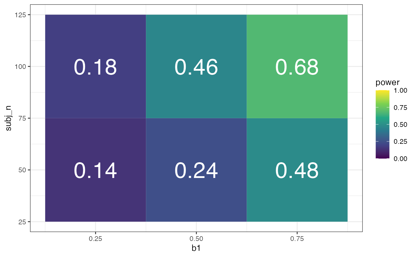
# calculate power for alpha = 0.05
filter(x, effect == "fixed", term == "cond.t") %>%
  group_by(b1, subj_n) %>%
  summarise(power = mean(p.value < .05),
            .groups = "drop") %>%
  ggplot(aes(b1, subj_n, fill = power)) +
  geom_tile() +
  geom_text(aes(label = sprintf("%.2f", power)), color = "white", size = 10) +
  scale_fill_viridis_c(limits = c(0, 1))