Appendix 1c: Sensitivity Analysis

Required software

# load required packages
library("lme4")        # model specification / estimation
library("lmerTest")    # deriving p-values from lmer
library("broom.mixed") # extracting data from model fits 
library("faux")        # generate correlated values
library("tidyverse")   # data wrangling and visualisation

# ensure this script returns the same results on each run
set.seed(8675309)
faux_options(verbose = FALSE)

Data simulation function

The custom simulation function for the example in Appendix 1A is copied below.

# set up the custom data simulation function
my_sim_data <- function(
  n_subj      = 100,   # number of subjects
  n_ingroup  =  25,   # number of ingroup stimuli
  n_outgroup =  25,   # number of outgroup stimuli
  beta_0     = 800,   # grand mean
  beta_1     =  50,   # effect of category
  omega_0    =  80,   # by-item random intercept sd
  tau_0      = 100,   # by-subject random intercept sd
  tau_1      =  40,   # by-subject random slope sd
  rho        = 0.2,   # correlation between intercept and slope
  sigma      = 200) { # residual (standard deviation)
  
  # simulate a sample of items
  items <- data.frame(
    item_id = seq_len(n_ingroup + n_outgroup),
    category = rep(c("ingroup", "outgroup"), c(n_ingroup, n_outgroup)),
    X_i = rep(c(-0.5, 0.5), c(n_ingroup, n_outgroup)),
    O_0i = rnorm(n = n_ingroup + n_outgroup, mean = 0, sd = omega_0)
  )

  # simulate a sample of subjects
  subjects <- faux::rnorm_multi(
    n = n_subj, mu = 0, sd = c(tau_0, tau_1), r = rho, 
    varnames = c("T_0s", "T_1s")
  )
  subjects$subj_id <- 1:n_subj
  
  # cross subject and item IDs 
  crossing(subjects, items)  %>%
    mutate(
      e_si = rnorm(nrow(.), mean = 0, sd = sigma),
      RT = beta_0 + T_0s + O_0i + (beta_1 + T_1s) * X_i + e_si
    ) %>%
    select(subj_id, item_id, category, X_i, RT)
}

Power calculation function

The power calculation function is slightly more complicated than the one for the basic example. Since sensitivity analyses usually push analyses into parameter spaces where the models produce warnings, we’re capturing the warnings and adding them to the results table. We’re also adding the parameters to the results table so you can group by the different parameter options when visualising the results.

# set up the power function
single_run <- function(filename = NULL, ...) {
  # ... is a shortcut that forwards any arguments to my_sim_data()
  dat_sim <- my_sim_data(...)

  # run lmer and capture any warnings
  ww <- ""
  suppressMessages(suppressWarnings(
    mod_sim <- withCallingHandlers({
      lmer(RT ~ X_i + (1 | item_id) + (1 + X_i | subj_id),
                  dat_sim, REML = FALSE)},
      warning = function(w) { ww <<- w$message }
    )
  ))
  
  # get results table and add rep number and any warnings
  sim_results <- broom.mixed::tidy(mod_sim) %>%
    mutate(warnings = ww)
  
  # add columns for the specified parameters
  params <- list(...)
  for (name in names(params)) {
    sim_results[name] <- params[name]
  }
  
  # append the results to a file if filename is set
  if (!is.null(filename)) {
    append <- file.exists(filename) # append if the file exists
    write_csv(sim_results, filename, append = append)
  }

  sim_results
}

Example 1: Effect size

Set up a data table with all of the parameter combinations you want to test. For example, the code below sets up 100 replications for effects of category ranging from 0 to 100 ms in steps of 10. All of the other parameters are default, but we’re specifying them anyways so they are saved in the results table.

filename1 <- "sims/sens1.csv"
nreps <- 100 # number of replications per parameter combo

params <- crossing(
  rep        = 1:nreps, # repeats each combo nreps times
  n_subj     = 100, # number of subjects
  n_ingroup  =  25, # number of ingroup stimuli
  n_outgroup =  25, # number of outgroup stimuli
  beta_0     = 800, # grand mean
  beta_1     = seq(0, 100, by = 10), # effect of category
  omega_0    = 100, # by-item random intercept sd
  tau_0      =  80, # by-subject random intercept sd
  tau_1      =  40, # by-subject random slope sd
  rho        = 0.2, # correlation between intercept and slope
  sigma      = 200  # residual (standard deviation)
) %>%
  select(-rep) # remove rep column

This table has 1100 rows, so will run 1100 simulations below. The code below saves the results to a named file or appends them to the file if one exists already. Run a small number of replicates to start and add to it after you’re sure your code works and you have an idea how long it takes.

if (!file.exists(filename1)) {
  # run a simulation for each row of params
  # and save to a file on each rep
  sims1 <- purrr::pmap_df(params, single_run, filename = filename1)
}

# read saved simulation data
# NB: col_types is set for warnings in case 
#     the first 1000 rows don't have any
ct <- cols(warnings = col_character(),
           # makes sure plots display in this order
           group = col_factor(ordered = TRUE),
           term = col_factor(ordered = TRUE))
sims1 <- read_csv(filename1, col_types = ct)

The chunk above will just read the saved data from the named file, if it exists. The code below calculates the mean estimates and power for each group. Make sure to set the group_by to the parameters you altered above.

# calculate mean estimates and power for specified alpha
alpha <- 0.05

power1 <- sims1 %>% 
  filter(effect == "fixed", term == "X_i") %>%
  group_by(term, beta_1) %>%
  summarise(
    mean_estimate = mean(estimate),
    mean_se = mean(std.error),
    power = mean(p.value < alpha),
    .groups = "drop"
  ) 

power1 %>%
  ggplot(aes(beta_1, power)) +
  geom_point() +
  geom_smooth(se = FALSE) +
  ylim(0, 1) +
  scale_x_continuous(name = "Effect of category in ms (beta_1)",
                     breaks = seq(0, 100, 10)) +
  ggtitle("Power for designs varying in effect size")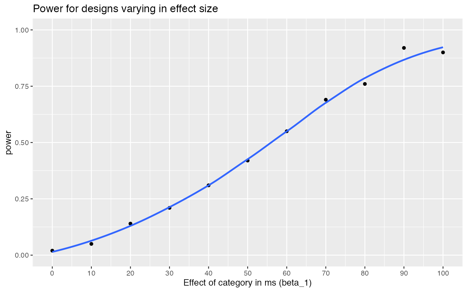

Example 2: Number of subjects and items

The code below sets up 50 replications for each of 20 combinations of 10 to 50 subjects (by steps of 10) and 10 to 25 stimuli (by steps of 5).

filename2 <- "sims/sens2.csv"
nreps <- 50 # number of replications per parameter combo

params <- crossing(
  rep       = 1:nreps, 
  n_subj    = seq(10, 50, by = 10),
  n_ingroup = seq(10, 25, by = 5),
  beta_0    = 800, # grand mean
  beta_1    = 100, # effect of category
  omega_0   = 100, # by-item random intercept sd
  tau_0     =  80, # by-subject random intercept sd
  tau_1     =  40, # by-subject random slope sd
  rho       = 0.2, # correlation between intercept and slope
  sigma     = 200  # residual (standard deviation)
) %>%
  mutate(n_outgroup = n_ingroup) %>%
  select(-rep) # remove rep column

if (!file.exists(filename2)) {
  # run a simulation for each row of params
  # and save to a file on each rep
  sims2 <- purrr::pmap_df(params, single_run, filename = filename2)
}

# read saved simulation data
sims2 <- read_csv(filename2, col_types = ct)

# calculate mean estimates and power for specified alpha
alpha <- 0.05

power2 <- sims2 %>% 
  filter(effect == "fixed", term == "X_i") %>%
  group_by(term, n_subj, n_ingroup) %>%
  summarise(
    mean_estimate = mean(estimate),
    mean_se = mean(std.error),
    power = mean(p.value < alpha),
    .groups = "drop"
  ) 

power2 %>%
  ggplot(aes(n_subj, n_ingroup, fill = power)) +
  geom_tile(show.legend = FALSE) +
  geom_text(aes(label = round(power, 2)), 
            color = "black", size = 6) +
  scale_x_continuous(name = "Number of subjects",
                     breaks = seq(10, 50, 10)) +
  scale_y_continuous(name = "Number of items/group",
                     breaks = seq(5, 25, 5)) +
  scale_fill_viridis_c(limits = c(0, 1)) +
  ggtitle("Power for designs varying in number of subjects and items")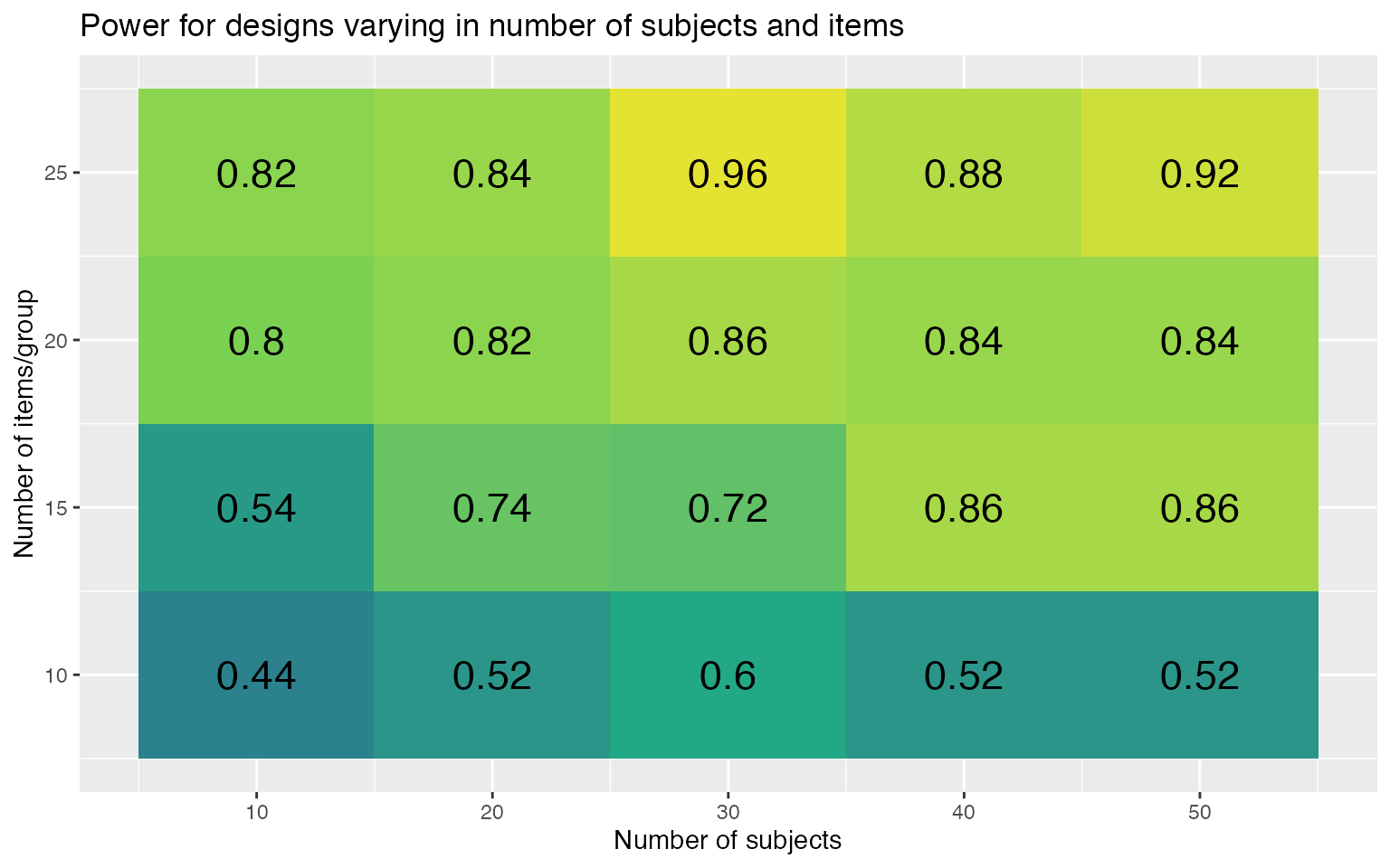

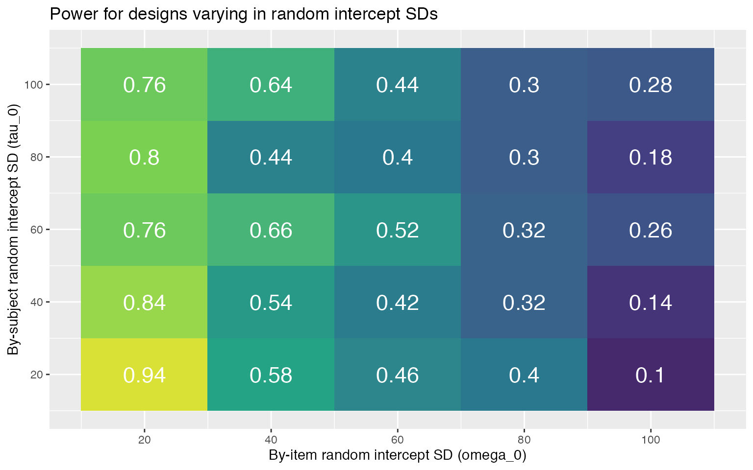
Example 3: Random intercept SDs

The code below sets up 50 replications for designs with 50 subjects, 10 items, and by-item and by-subject random intercept SDs ranging from 20 to 100 in steps of 20.

filename3 <- "sims/sens3.csv"
nreps <- 50 # number of replications per parameter combo

params <- crossing(
  rep        = 1:nreps,
  n_subj     =  50, # number of subjects
  n_ingroup  =  10, # number of ingroup items
  n_outgroup =  10, # number of outgroup items
  beta_0     = 800, # grand mean
  beta_1     =  50, # effect of category
  omega_0    = seq(20, 100, by = 20), # by-item random intercept sd
  tau_0      = seq(20, 100, by = 20), # by-subject random intercept sd
  tau_1      =  40, # by-subject random slope sd
  rho        = 0.2, # correlation between intercept and slope
  sigma      = 200  # residual (standard deviation)
) %>%
  select(-rep) # remove rep column

if (!file.exists(filename3)) {
  # run a simulation for each row of params
  # and save to a file on each rep
  sims3 <- purrr::pmap_df(params, single_run, filename = filename3)
}

# read saved simulation data
sims3 <- read_csv(filename3, col_types = ct)

# calculate mean estimates and power for specified alpha
alpha <- 0.05

power3 <- sims3 %>% 
  filter(effect == "fixed", term == "X_i") %>%
  group_by(term, omega_0, tau_0) %>%
  summarise(
    mean_estimate = mean(estimate),
    mean_se = mean(std.error),
    power = mean(p.value < alpha),
    .groups = "drop"
  ) 

power3 %>%
  ggplot(aes(omega_0, tau_0, fill = power)) +
  geom_tile(show.legend = FALSE) +
  geom_text(aes(label = round(power, 2)), 
            color = "white", size = 6) +
  scale_x_continuous(name = "By-item random intercept SD (omega_0)",
                     breaks = seq(20, 100, 20)) +
  scale_y_continuous(name = "By-subject random intercept SD (tau_0)",
                     breaks = seq(20, 100, 20)) +
  scale_fill_viridis_c(limits = c(0, 1)) +
  ggtitle("Power for designs varying in random intercept SDs")