Appendix 3a: Binomial Example
Understanding mixed effects models through data simulation
Lisa M. DeBruine & Dale J. Barr
Source:vignettes/appendix3a_binomial.Rmd
appendix3a_binomial.RmdDownload the .Rmd for this example
Simulating binomial data with crossed random factors
To give an overview of the simulation task, we will simulate data from a design with crossed random factors of subjects and stimuli, fit a model to the simulated data, and then try to recover the parameter values we put in from the output. In this hypothetical study, subjects classify the emotional expressions of faces as quickly as possible, and we use accuracy (correct/incorrect) as the primary dependent variable. The faces are of two types: either from the subject’s ingroup or from an outgroup. For simplicity, we further assume that each face appears only once in the stimulus set. The key question is whether there is any difference in classification accuracy across the type of face.
The important parts of the design are:
- Random factor 1: subjects (associated variables will be prefixed by T, \(\tau\), or
tau) - Random factor 2: faces (associated variables will be prefixed by O, \(\omega\), or
omega) - Fixed factor 1: category (level = ingroup, outgroup)
- within subject: subjects see both ingroup and outgroup faces
- between face: faces are either ingroup or outgroup
Required software
# load required packages
library("lme4")        # model specification / estimation
library("afex")        # anova and deriving p-values from lmer
library("broom.mixed") # extracting data from model fits
library("faux")        # data simulation
library("tidyverse")   # data wrangling and visualisation

# ensure this script returns the same results on each run
set.seed(8675309)
faux_options(verbose = FALSE)
This example presents a simulation for a binomial logistic mixed regression. Part of the process involves conversion between probability and the logit function of probability. The code below converts between these.
logit <- function(x) { log(x / (1 - x)) }
inv_logit <- function(x) { 1 / (1 + exp(-x)) }

data.frame(
  prob = seq(0,1,.01)
) %>%
  mutate(logit = logit(prob)) %>%
  ggplot(aes(prob, logit)) +
  geom_point()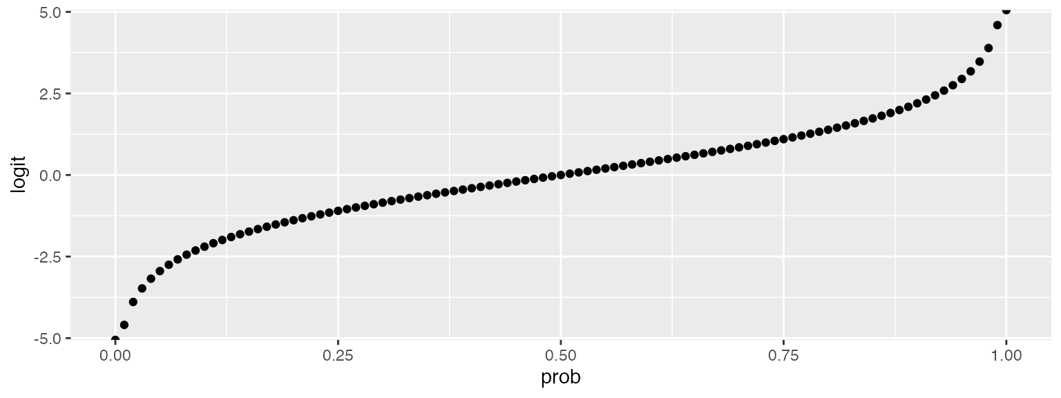
Data simulation function
The data generating process is slighly different for binomial logistic regression. The random effects and their correlations are set the same way as for a gaussian model (you’ll need some pilot data to estimate reasonable parameters), but we don’t need an error term.
# set up the custom data simulation function
my_bin_data <- function(
  n_subj     = 100, # number of subjects
  n_ingroup  =  25,  # number of faces in ingroup
  n_outgroup =  25,  # number of faces in outgroup
  beta_0     =   0, # intercept
  beta_1     =   0, # effect of category
  omega_0    =   1, # by-item random intercept sd
  tau_0      =   1, # by-subject random intercept sd
  tau_1      =   1, # by-subject random slope sd
  rho        =   0 # correlation between intercept and slope
                        ) {
   # simulate a sample of items
  items <- data.frame(
    item_id = 1:(n_ingroup + n_outgroup),
    category = rep(c("ingroup", "outgroup"),
                   c(n_ingroup, n_outgroup)),
    O_0i = rnorm(n_ingroup + n_outgroup, 0, omega_0)
  )

  # effect code category
  items$X_i <- recode(items$category,
                      "ingroup" = -0.5,
                      "outgroup" = 0.5)

  # simulate a sample of subjects
  subjects <- faux::rnorm_multi(
    n = n_subj,
    mu = 0,
    sd = c(tau_0, tau_1),
    r = rho,
    varnames = c("T_0s", "T_1s")
  )
  subjects$subj_id <- 1:n_subj

  # cross subject and item IDs
  crossing(subjects, items)  %>%
    mutate(
      # calculate gaussian DV
      Y = beta_0 + T_0s + O_0i + (beta_1 + T_1s) * X_i,
      pr = inv_logit(Y), # transform to probability of getting 1
      Y_bin = rbinom(nrow(.), 1, pr) # sample from bernoulli distribution
    ) %>%
    select(subj_id, item_id, category, X_i, Y, Y_bin)
}
dat_sim <- my_bin_data()
head(dat_sim)
## # A tibble: 6 x 6
## subj_id item_id category X_i Y Y_bin
## <int> <int> <chr> <dbl> <dbl> <int>
## 1 63 1 ingroup -0.5 -3.60 0
## 2 63 2 ingroup -0.5 -1.88 0
## 3 63 3 ingroup -0.5 -3.22 0
## 4 63 4 ingroup -0.5 -0.576 0
## 5 63 5 ingroup -0.5 -1.54 0
## 6 63 6 ingroup -0.5 -1.62 0Power function
single_run <- function(filename = NULL, ...) {
  # ... is a shortcut that forwards any arguments to my_sim_data()
  dat_sim <- my_bin_data(...)
  mod_sim <- glmer(Y_bin ~ 1 + X_i + (1 | item_id) + (1 + X_i | subj_id),
                data = dat_sim, family = "binomial")

  sim_results <- broom.mixed::tidy(mod_sim)

  # append the results to a file if filename is set
  if (!is.null(filename)) {
    append <- file.exists(filename) # append if the file exists
    write_csv(sim_results, filename, append = append)
  }

  # return the tidy table
  sim_results
}
# run one model with default parameters
single_run()
## # A tibble: 6 x 7
## effect group term estimate std.error statistic p.value
## <chr> <chr> <chr> <dbl> <dbl> <dbl> <dbl>
## 1 fixed <NA> (Intercept) -0.0343 0.166 -0.207 0.836
## 2 fixed <NA> X_i 0.0670 0.292 0.230 0.818
## 3 ran_pars subj_id sd__(Intercept) 0.942 NA NA NA
## 4 ran_pars subj_id cor__(Intercept).X_i -0.0466 NA NA NA
## 5 ran_pars subj_id sd__X_i 1.01 NA NA NA
## 6 ran_pars item_id sd__(Intercept) 0.938 NA NA NAThe following function converts probabilities of getting a 1 in the first and second category levels into beta values. You will need to figure out a custom function for each design to do this, or estimate fixed effect parameters from analysis of pilot data.
prob2param <- function(a = 0, b = 0) {
  list(
    beta_0 = (logit(a) + logit(b))/2,
    beta_1 = logit(a) - logit(b)
  )
}
To get an accurate estimation of power, you need to run the simulation many times. We use 20 here as an example because the analysis is very slow, but your results are more accurate the more replications you run. This will depend on the specifics of your analysis, but we recommend at least 1000 replications.
# run simulations and save to a file on each rep
filename <- "sims/binomial.csv"
reps <- 20
b <- prob2param(.4, .6)
tau_0    <- 1
tau_1    <- 1
omega_0  <- 1
rho      <- 0.5

if (!file.exists(filename)) {
  # run simulations and save to a file
  sims <- purrr::map_df(1:reps, ~single_run(
    filename = filename,
    beta_0   = b$beta_0,
    beta_1   = b$beta_1,
    tau_0    = tau_0,
    tau_1    = tau_1,
    omega_0  = omega_0,
    rho      = 0.5)
  )
}

# read saved simulation data
ct <- cols(# makes sure plots display in this order
           group = col_factor(ordered = TRUE),
           term = col_factor(ordered = TRUE))
sims <- read_csv(filename, col_types = ct)
Calculate mean estimates and cell probabilities
est <- sims %>%
  group_by(group, term) %>%
  summarise(
    mean_estimate = mean(estimate),
    .groups = "drop"
  )

int_est <- filter(est, is.na(group), term == "(Intercept)") %>%
  pull(mean_estimate)
cat_est <- filter(est, is.na(group), term == "X_i") %>%
  pull(mean_estimate)

pr0 <- inv_logit(int_est) %>% round(2)
pr1_plus <- inv_logit(int_est + .5*cat_est) %>% round(2)
pr1_minus <- inv_logit(int_est - .5*cat_est) %>% round(2)

est %>%
  arrange(!is.na(group), group, term) %>%
  mutate(
  sim = c(b$beta_0, b$beta_1, omega_0, rho, tau_0, tau_1),
  prob = c(pr0, paste0(pr1_minus, ":", pr1_plus), rep(NA, 4))
) %>%
  mutate_if(is.numeric, round, 2)
## # A tibble: 6 x 5
## group term mean_estimate sim prob
## <ord> <ord> <dbl> <dbl> <chr>
## 1 <NA> (Intercept) -0.04 0 0.49
## 2 <NA> X_i -0.86 -0.81 0.6:0.39
## 3 subj_id sd__(Intercept) 1.02 1 <NA>
## 4 subj_id cor__(Intercept).X_i 0.5 0.5 <NA>
## 5 subj_id sd__X_i 1.02 1 <NA>
## 6 item_id sd__(Intercept) 0.99 1 <NA>