Appendix 3b: Extended Binomial Example
Simulating binomial data with crossed random factors
Lisa M. DeBruine, Dorothy Bishop, Dale J. Barr
Source:vignettes/appendix3b_extended_binomial.Rmd
appendix3b_extended_binomial.RmdDownload the .Rmd for this example
To give an overview of the simulation task, we will simulate data from a design with crossed random factors of subjects and stimuli, fit a model to the simulated data, and then try to recover the parameter values we put in from the output. In this hypothetical study, subjects classify the emotional expressions of faces as quickly as possible, and we use accuracy (correct/incorrect) as the primary dependent variable. The faces are of two types: either from the subject’s ingroup or from an outgroup. The key question is whether there is any difference in classification accuracy across the type of face.
The important parts of the design are:
- Random factor 1: subjects
- Random factor 2: faces
- Fixed factor 1: expression (level = angry, happy)
- within subject: same subjects see both angry and happy faces
- within face: same faces are both angry and happy
- Fixed factor 2: category (level = ingroup, outgroup)
- within subject: same subjects see both ingroup and outgroup faces
- between face: each face is either ingroup or outgroup
Required software
# load required packages
library("lme4")        # model specification / estimation
library("afex")        # deriving p-values from lmer
library("broom.mixed") # extracting data from model fits
library("faux")        # data simulation for multivariate normal dist
library("tidyverse")   # data wrangling and visualisation
# ensure this script returns the same results on each run
set.seed(8675309)
faux_options(verbose = FALSE)
Probability vs logit
This example presents an extended simulation for a binomial logistic mixed regression. Where response accuracy is measured in terms of probability, the regression needs to work with a link function that uses the logit, which does not have the problems of being bounded by 0 and 1. The functions below are used later to convert between probability and the logit function of probability.
logit <- function(x) { log(x / (1 - x)) }

inv_logit <- function(x) { 1 / (1 + exp(-x)) }

data.frame(
  prob = seq(0,1,.01)
) %>%
  mutate(logit = logit(prob)) %>%
  ggplot(aes(prob, logit)) +
  geom_point()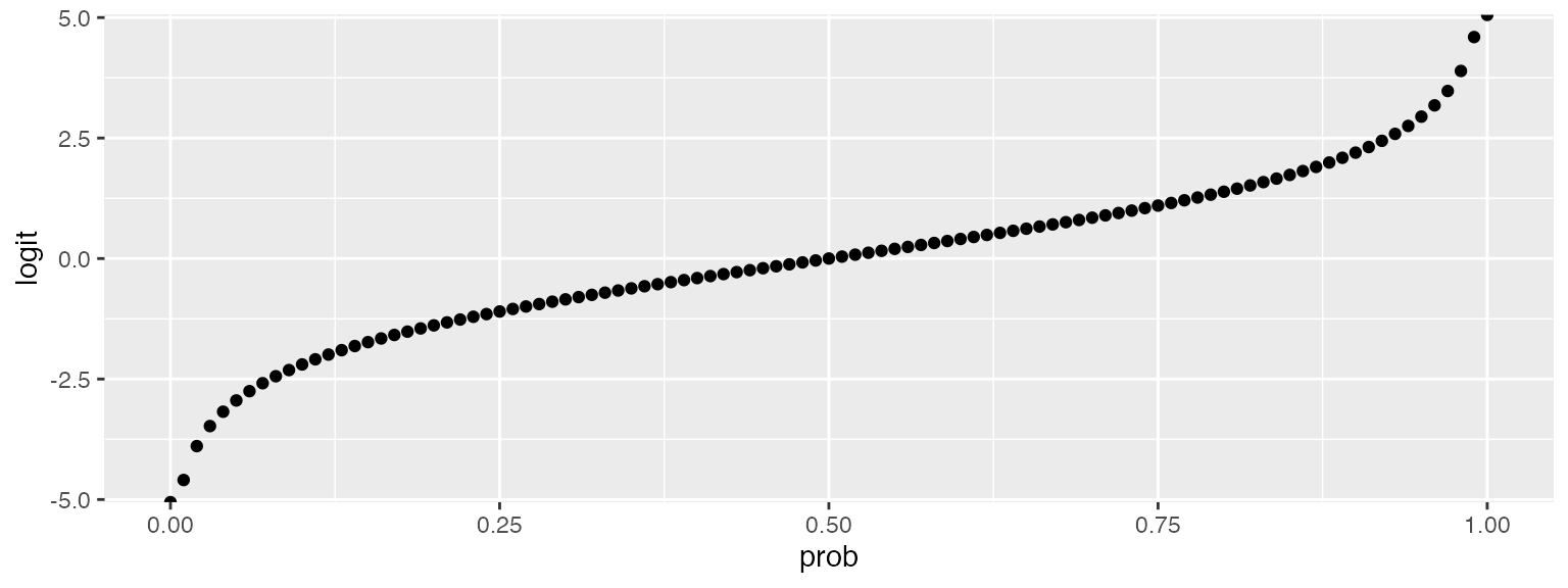
2ww*2wb design
In this example, 30 subjects will respond twice (for happy and angry expressions) to 50 items; 25 items in each of 2 categories. In this example, expression is a within-subject and within-item factor and category is a within-subject and between-item factor.
Terms
We use the following prefixes to designate model parameters and sampled values:
-
beta_*: fixed effect parameters -
subj_*: random effect parameters associated with subjects -
item_*: random effect parameters associated with items -
X_*: effect-coded predictor -
S_*: sampled values for subject random effects -
I_*: sampled values for item random effects
In previous tutorials, we used numbers to designate fixed effects, but here we will use letter abbreviations to make things clearer:
-
*_0: intercept -
*_e: expression -
*_c: category -
*_ec: expression * category
Other terms:
-
*_rho: correlations; a vector of the upper right triangle for the correlation matrix for that group’s random effects -
n_*: sample size
Data-generating function
Betas are on logit scale; later we use inv_logit() to convert to probabilities. The defaults for the data-generating function ext_bin_dgf() are for null effects. When simulating realistic data, we will call the function using beta values computed using expected probabilities for combinations of independent variables, which will overwrite the defaults specified here. All SDs, representing variation in item and subject-specific effects, are set to one.
ext_bin_dgf <- function(
  n_subj     =  30, # number of subjects
  n_ingroup  =  25, # number of faces in ingroup
  n_outgroup =  25, # number of faces in outgroup
  beta_0     =   0, # grand mean - inv_logit(0)=.5
  beta_e     =   0, # main effect of expression
  beta_c     =   0, # main effect of category
  beta_ec    =   0, # interaction between category and expression
  item_0     =   1, # by-item random intercept sd
  item_e     =   1, # by-item random slope for exp
  item_rho   =   0, # by-item random effect correlation
  subj_0     =   1, # by-subject random intercept sd
  subj_e     =   1, # by-subject random slope sd for exp
  subj_c     =   1, # by-subject random slope sd for category
  subj_ec    =   1, # by-subject random slope sd for category*exp
  # by-subject random effect correlations
  subj_rho   = c(0, 0, 0, # subj_0  * subj_e, subj_c, subj_ec
                    0, 0, # subj_e  *         subj_c, subj_ec
                       0) # subj_c  *                 subj_ec
) {
  # simulate items;  separate item ID for each item;
  # simulating each item's individual effect for intercept (I_0)
  #   and slope (I_e) for expression (the only within-item factor)
  items <- faux::rnorm_multi(
    n = n_ingroup + n_outgroup,
    mu = 0,
    sd = c(item_0, item_e),
    r = item_rho,
    varnames = c("I_0", "I_e")
  ) %>%
    mutate(item_id = faux::make_id(nrow(.), "I"),
           category = rep(c("ingroup", "outgroup"),
                           c(n_ingroup, n_outgroup))) %>%
    select(item_id, category, everything())

  # simulate subjects: separate subject ID for each subject;
  # simulating each subject's individual effect for intercept (I_0)
  #   and slope for each within-subject factor and their interaction.
  subjects <- faux::rnorm_multi(
    n = n_subj,
    mu = 0,
    sd = c(subj_0, subj_e, subj_c, subj_ec),
    r = subj_rho,
    varnames = c("S_0", "S_e", "S_c", "S_ec")
  ) %>%
    mutate(subj_id = faux::make_id(nrow(.), "S")) %>%
    select(subj_id, everything())

  # simulate trials
  crossing(subjects, items,
    expression = factor(c("happy", "angry"), ordered = TRUE)
  ) %>%
    mutate(
      # effect code the two fixed factors
      X_e = recode(expression, "happy" = -0.5, "angry" = 0.5),
      X_c = recode(category, "ingroup" = -0.5, "outgroup" = +0.5),
      # add together fixed and random effects for each effect
      B_0  = beta_0  + S_0 + I_0,
      B_e  = beta_e  + S_e + I_e,
      B_c  = beta_c  + S_c,
      B_ec = beta_ec + S_ec,
      # calculate gaussian effect
      Y = B_0 + (B_e*X_e) + (B_c*X_c) + (B_ec*X_e*X_c),
      pr = inv_logit(Y), # transform to probability of getting 1
      Y_bin = rbinom(nrow(.), 1, pr) # sample from bernoulli distribution, ie use pr to set observed binary response to 0 or 1, so if pr = .5, then 0 and 1 equally likely
    ) %>%
    select(subj_id, item_id, expression, category, X_e, X_c, Y, Y_bin)
}
You can set the subject and item Ns to very small numbers to check that the design is what you expect. Here, we have two subjects who each see two faces, one ingroup and one outgroup, in each of two expressions, happy and angry, for a total of four trials per subject.
ext_bin_dgf(n_subj = 2, n_ingroup = 1, n_outgroup = 1)## # A tibble: 8 x 8
## subj_id item_id expression category X_e X_c Y Y_bin
## <chr> <chr> <ord> <chr> <dbl> <dbl> <dbl> <int>
## 1 S1 I1 angry ingroup 0.5 -0.5 -1.42 0
## 2 S1 I1 happy ingroup -0.5 -0.5 -0.467 1
## 3 S1 I2 angry outgroup 0.5 0.5 -2.65 0
## 4 S1 I2 happy outgroup -0.5 0.5 -4.48 0
## 5 S2 I1 angry ingroup 0.5 -0.5 1.01 1
## 6 S2 I1 happy ingroup -0.5 -0.5 1.60 1
## 7 S2 I2 angry outgroup 0.5 0.5 0.389 0
## 8 S2 I2 happy outgroup -0.5 0.5 -1.73 0Single run
The single_run() function creates a simulated data set using the ext_bin_dgf() function, runs a GLMM analysis, and returns a tidy table of the results. If you set filename, it will also record the data to a file, which can be helpful if you need to run a long simulation that might crash or you might need to interrupt.
single_run <- function(filename = NULL, ...) {
  # ... represents additional arguments to be passed to ext_bin_dgf
  dat_sim <- ext_bin_dgf(...)
  mod_sim <- glmer(Y_bin ~ 1 + X_e*X_c +
                     (1 + X_e | item_id) +
                     (1 + X_e*X_c | subj_id),
                data = dat_sim, family = "binomial")

  sim_results <- broom.mixed::tidy(mod_sim)

  # append the results to a file if filename is set
  if (!is.null(filename)) {
    append <- file.exists(filename) # append if the file exists
    write_csv(sim_results, filename, append = append)
  }

  # return the tidy table
  sim_results
}
You can compare a single run output with the parameters that were set. However, unless your Ns are very big, expect a few large deviations by chance. Run this function once with a timing function to see how long it takes. Mixed model simulations can take a long time, so knowing this lets you figure out how long your coffee break can be when you run the simulation below.
system.time(
  s <- single_run()
)
## user system elapsed
## 14.977 0.062 15.069
s## # A tibble: 17 x 7
## effect group term estimate std.error statistic p.value
## <chr> <chr> <chr> <dbl> <dbl> <dbl> <dbl>
## 1 fixed <NA> (Intercept) 0.109 0.286 0.382 0.703
## 2 fixed <NA> X_e -0.0360 0.234 -0.154 0.878
## 3 fixed <NA> X_c -0.128 0.362 -0.353 0.724
## 4 fixed <NA> X_e:X_c 0.0192 0.350 0.0547 0.956
## 5 ran_pars item_id sd__(Intercept) 1.03 NA NA NA
## 6 ran_pars item_id cor__(Intercept).X_e -0.142 NA NA NA
## 7 ran_pars item_id sd__X_e 0.675 NA NA NA
## 8 ran_pars subj_id sd__(Intercept) 1.32 NA NA NA
## 9 ran_pars subj_id cor__(Intercept).X_e -0.373 NA NA NA
## 10 ran_pars subj_id cor__(Intercept).X_c 0.396 NA NA NA
## 11 ran_pars subj_id cor__(Intercept).X_e:X… 0.0376 NA NA NA
## 12 ran_pars subj_id sd__X_e 1.05 NA NA NA
## 13 ran_pars subj_id cor__X_e.X_c -0.178 NA NA NA
## 14 ran_pars subj_id cor__X_e.X_e:X_c -0.00909 NA NA NA
## 15 ran_pars subj_id sd__X_c 1.05 NA NA NA
## 16 ran_pars subj_id cor__X_c.X_e:X_c -0.219 NA NA NA
## 17 ran_pars subj_id sd__X_e:X_c 1.23 NA NA NACalculate betas from probabilities
The following function calculates the betas (on a logit scale) from the mean probability correct for each combination of factors. The default is all are 50% correct.
This function only works for a 2x2 design like the one in this example. You will need to figure out a custom function for each design to do this, or estimate fixed effect parameters directly from analysis of pilot data.
# set level 1 for each factor to the +0.5-coded value

prob2param <- function(A1B1 = .5,   # angry outgroup
                       A1B2 = .5,   # angry ingroup
                       A2B1 = .5,   # happy outgroup
                       A2B2 = .5) { # happy ingroup
  # convert probabilities to logit
  a1b1 <- logit(A1B1)
  a1b2 <- logit(A1B2)
  a2b1 <- logit(A2B1)
  a2b2 <- logit(A2B2)

  # calculate and return betas
  list(
    beta_0 = mean(c(a1b1, a1b2, a2b1, a2b2)), # grand mean
    beta_e = (a1b1+a1b2)/2 - (a2b1+a2b2)/2, # angry - happy
    beta_c = (a1b1+a2b1)/2 - (a1b2+a2b2)/2, # outgroup - ingroup
    beta_ec = (a1b1-a1b2) - (a2b1-a2b2) # angry o-i diff - happy o-i diff
  )
}
Demonstrate a single run of the function. First we specify proportions correct for the 4 combinations. These are just made-up values to show how it works. With values set to .6, .5, .5, and .4,, we get beta_0 and beta_ec of 0 (no interaction), and beta_e and beta_c of .405 (same size effect of angry/happy and ingroup/outgroup).
# to check false positive rate of analysis, set all these to same value (e.g. .5)
A1B1 <- .6 # angry_outgroup
A1B2 <- .5 # angry_ingroup
A2B1 <- .5 # happy_outgroup
A2B2 <- .4 # happy_ingroup
b <- prob2param(A1B1, A1B2, A2B1, A2B2)
str(b)
## List of 4
## $ beta_0 : num -1.39e-17
## $ beta_e : num 0.405
## $ beta_c : num 0.405
## $ beta_ec: num -5.55e-17Simulations
We can now run many simulations and save to a file on each run. It’s a good idea to put the relevant parameters in the filename, or modify the code above to add the parameters as new columns.
# make a filename indicating this specific set of estimated values
filename <- paste0("sims/binomial_ext_",A1B1,"_",A1B2,"_",A2B1,"_",A2B2,".csv")
This can take a very long time, so set eval = FALSE to skip this chunk if you’ve already run it and just load the data from the file. Alternatively, as below, surround the simulation code with a conditional statement to only run if the file isn’t already present.
If you want to add additional reps to your file, make sure you change the seed, or each time your run this script from the start, you’ll just get identical numbers.
reps <- 10
# run simulations and save to a file

if (!file.exists(filename)) {
  sims <- purrr::map_df(1:reps, ~single_run(
    filename = filename,
    beta_0 = b$beta_0,
    beta_e = b$beta_e,
    beta_c = b$beta_c,
    beta_ec = b$beta_ec)
  )
}
# read saved simulation data
sims <- read_csv(filename)
Calculate mean estimates and power
-
mean_estimateis the mean estimate of that value in the simulations -
poweris the proportion of alpha values for each fixed effect that are less than your alpha (here set to .05). -
sim_valueis the true value of beta derived from the probabilities we specified
alpha <- 0.05 # justify your alpha

est <- sims %>%
  dplyr::filter(effect == "fixed") %>%
  dplyr::group_by(term) %>%
  dplyr::summarise(
    mean_estimate = mean(estimate),
    power = mean(p.value < alpha),
    .groups = "drop"
  )

# Note use of dplyr:: with some tidyverse commands to avoid problems that can arise from conflicts of these names with other packages.

est %>% mutate(
  parameter = c("beta_0", "beta_c", "beta_e", "beta_ec"),
  sim_value = c(b$beta_0, b$beta_c, b$beta_e, b$beta_ec)
) %>%
  mutate_if(is.numeric, round, 4)
## # A tibble: 4 x 5
## term mean_estimate power parameter sim_value
## <chr> <dbl> <dbl> <chr> <dbl>
## 1 (Intercept) 0.0354 0.1 beta_0 0
## 2 X_c 0.373 0.4 beta_c 0.406
## 3 X_e 0.491 0.6 beta_e 0.406
## 4 X_e:X_c -0.102 0 beta_ec 0Calculate probabilities
Sum estimates for each cell and use inverse logit transform to recover probabilities. Compare with the values of A1B1 … A2B2 used to calculate the simulation parameters.
# get estimates of beta values
int <- est[[1,2]]
cat <- est[[2,2]]
exp <- est[[3,2]]
cat_exp <- est[[4,2]]

# effect-coding of factor levels
happy <- -0.5
angry <- +0.5
ig    <- -0.5
og    <- +0.5

data.frame(
  angry_outgroup = int + og*cat + angry*exp + og*angry*cat_exp,
  angry_ingroup  = int + ig*cat + angry*exp + ig*angry*cat_exp,
  happy_outgroup = int + og*cat + happy*exp + og*happy*cat_exp,
  happy_ingroup  = int + ig*cat + happy*exp + ig*happy*cat_exp
) %>%
  gather(key, estimate, 1:4) %>%
  mutate(estimate = inv_logit(estimate)) %>%
  mutate(prob = c(A1B1, A1B2, A2B1, A2B2)) %>%
  separate(key, c("exp", "cat")) %>%
  mutate_if(is.numeric, round, 2)
## exp cat estimate prob
## 1 angry outgroup 0.61 0.6
## 2 angry ingroup 0.53 0.5
## 3 happy outgroup 0.50 0.5
## 4 happy ingroup 0.40 0.4