Appendix 2: Extended Examples
Understanding mixed effects models through data simulation
Lisa M. DeBruine & Dale J. Barr
Source:vignettes/appendix2_extended_example.Rmd
appendix2_extended_example.RmdDownload the .Rmd for this example
library("lme4")        # model specification / estimation
library("afex")        # deriving p-values from lmer
library("broom.mixed") # extracting data from model fits
library("faux")        # data simulation
library("tidyverse")   # data wrangling and visualisation

# ensure this script returns the same results on each run
set.seed(90210)
faux_options(verbose = FALSE)
2ww2wb Design
This section will simulate data and run a power analysis for a 2x2 design where the first factor is within subjects and within items and the second factor is with subjects and between items.
Set Study Parameters
In this example, 50 subjects will respond twice (for happy and angry expressions) to 50 items; 25 items in each of 2 categories. In this example, expression is a within-subject and within-item factor and category is a within-subject and between-item factor.
We will set our grand intercept and the fixed effect of category the same as before (800 ms and 50ms). We will predict that classification speed will be faster for angry than happy outgroup faces, and faster for happy than angry ingroup faces. In other words, the effect of category will be bigger for happy faces than angry faces, but there will be no main effect of expression, just an interaction between category and expression, which we will set at 70 ms (the 50ms effect of category will be 35 ms bigger for happy faces and 35 ms smaller for angry faces).
Therefore, you will need to set up more complicated random effect parameters. Items and subjects will need standard deviations assigned for their random intercepts and the random slopes for any within factors (and their interactions), plus the correlations among all these SDs.
Since all subjects respond to all items, we can set up a table of trials by crossing the subject IDs with the item IDs and also any factors that are both within-subject and within-item (i., expression = c("happy", "angry")). This is set up as a factor with the levels specified so they are displayed in the right order in plots.
We use the following prefixes to designate model parameters and sampled values: * beta_*: fixed effect parameters * subj_*: random effect parameters associated with subjects * item_*: random effect parameters associated with items * X_*: effect-coded predictor * S_*: sampled values for subject random effects * I_*: sampled values for item random effects
In previous tutorials, we used numbers to designate fixed effects, but here we will use letter abbreviations to make things clearer:
-
*_0: intercept -
*_e: expression -
*_c: category -
*_ec: expression * category
Other terms:
-
*_rho: correlations; a vector of the upper right triangle for the correlation matrix for that group’s random effects -
n_*: sample size -
sigma: residual (error) sd
# data simulation for a design with a 2x2 design where
# the first factor is within subjects and within items,
# and the second factor is within subjects and between items

sim_data_2ww2wb <- function(
  n_subj     =  50, # number of subjects
  n_ingroup  =  25, # number of items in ingroup
  n_outgroup =  25, # number of items in outgroup
  beta_0     = 800, # intercept (grand mean)
  beta_e     =  50, # main effect of category
  beta_c     =   0, # main effect of expression
  beta_ec    =  70, # interaction between category and expression
  subj_0     = 100, # by-subject random intercept sd
  subj_e     =  40, # by-subject random slope sd for exp
  subj_c     =  80, # by-subject random slope sd for category
  subj_ec    =  80, # by-subject random slope sd for category*exp
  # by-subject random effect correlations
  subj_rho   = c(.3, .3, .3,   # beta_0 * beta_c, beta_e, beta_ce
                     .1, .1,   # beta_c *         beta_e, beta_ce
                         .1),  # beta_e *                 beta_ce
  item_0     =  80, # by-item random intercept sd
  item_e     =  60, # by-item random slope for exp
  item_rho   = 0.2, # by-item random effect correlations
  sigma      = 200   # residual (error) sd
) {

  # simulate items
  items <- faux::rnorm_multi(
    n = n_ingroup + n_outgroup,
    mu = 0,
    sd = c(item_0, item_e),
    r = item_rho,
    varnames = c("I_0", "I_e")
  ) %>%
    mutate(item_id = faux::make_id(nrow(.), "I"),
           category = rep(c("ingroup", "outgroup"),
                           c(n_ingroup, n_outgroup)))

  # simulate subjects
  subjects <- faux::rnorm_multi(
    n = n_subj,
    mu = 0,
    sd = c(subj_0, subj_e, subj_c, subj_ec),
    r = subj_rho,
    varnames = c("S_0", "S_e", "S_c", "S_ec")
  ) %>%
    mutate(subj_id = faux::make_id(nrow(.), "S"))

  # simulate trials
  crossing(subjects, items,
    expression = factor(c("happy", "angry"), ordered = TRUE)
  ) %>%
    mutate(
      # effect code the two fixed factors
      X_e = recode(expression, "happy" = -0.5, "angry" = 0.5),
      X_c = recode(category, "ingroup" = -0.5, "outgroup" = +0.5),
      # add together fixed and random effects for each effect
      B_0  = beta_0  + S_0 + I_0,
      B_e  = beta_c  + S_e + I_e,
      B_c  = beta_e  + S_c,
      B_ec = beta_ec + S_ec,
      # generate the error term
      e_si = rnorm(nrow(.), mean = 0, sd = sigma),
      # calculate RT by adding each effect term
      # multiplied by the relevant effect-coded factor(s)
      RT = B_0 + (B_e*X_e) + (B_c*X_c) + (B_ec*X_e*X_c) + e_si
    ) %>%
    select(subj_id, item_id, expression, category, X_e, X_c, RT)
}
Plot your data to double-check it looks like you expect.
dat_sim <- sim_data_2ww2wb()

ggplot(dat_sim, aes(expression, RT, color = category)) +
  geom_boxplot(width = 0.25, position = position_dodge(width = 0.9))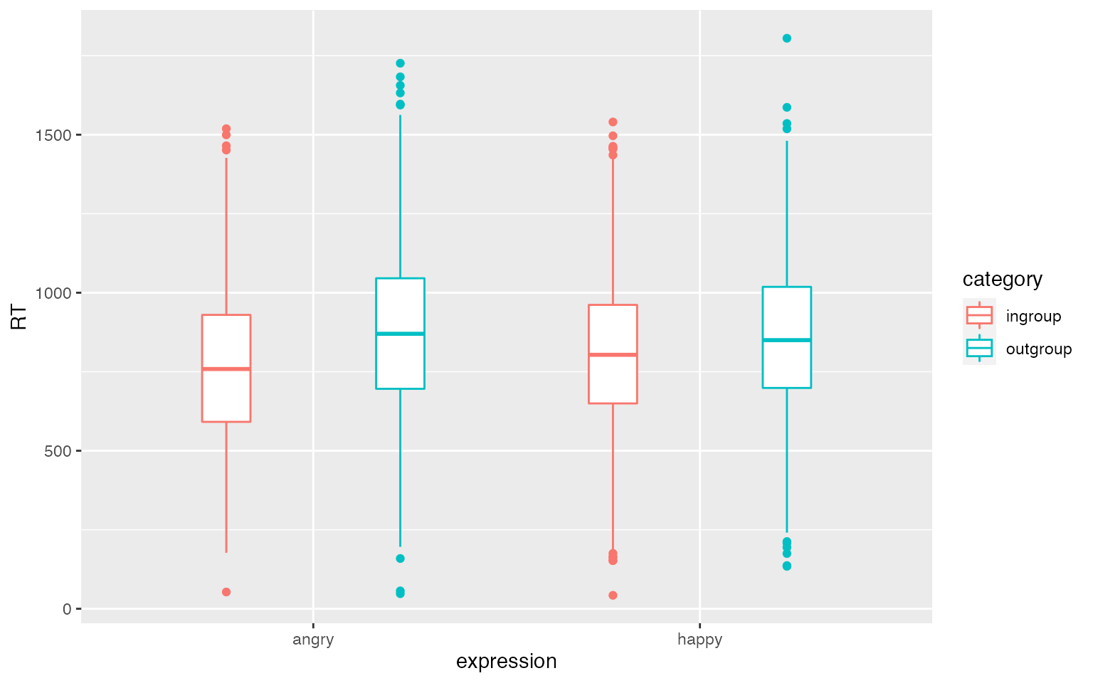
Analyse Data
# set up the power function
single_run <- function(filename = NULL, ...) {
  dat_sim <- sim_data_2ww2wb(...)

  mod_sim <- lmer(RT ~ 1 + X_e*X_c +
                    (1 + X_e | item_id) +
                    (1 + X_e*X_c | subj_id),
                  data = dat_sim)

  sim_results <- broom.mixed::tidy(mod_sim)

  # append the results to a file if filename is set
  if (!is.null(filename)) {
    append <- file.exists(filename) # append if the file exists
    write_csv(sim_results, filename, append = append)
  }

  # return the tidy table
  sim_results
}
Run the function once with default parameters. If you run it between two calls to Sys.time(), you can find out how long one run takes (this can be a long time for complex designs).
start_time <- Sys.time()
single_run()
## # A tibble: 18 x 8
## effect group term estimate std.error statistic df p.value
## <chr> <chr> <chr> <dbl> <dbl> <dbl> <dbl> <dbl>
## 1 fixed <NA> (Intercept) 778. 18.3 42.6 80.9 3.52e-57
## 2 fixed <NA> X_e 4.00 11.9 0.337 51.4 7.38e- 1
## 3 fixed <NA> X_c 79.5 24.1 3.30 77.0 1.48e- 3
## 4 fixed <NA> X_e:X_c 76.0 26.6 2.86 65.8 5.74e- 3
## 5 ran_pars item_… sd__(Intercept) 69.3 NA NA NA NA
## 6 ran_pars item_… cor__(Intercept… -0.104 NA NA NA NA
## 7 ran_pars item_… sd__X_e 70.1 NA NA NA NA
## 8 ran_pars subj_… sd__(Intercept) 107. NA NA NA NA
## 9 ran_pars subj_… cor__(Intercept… 0.199 NA NA NA NA
## 10 ran_pars subj_… cor__(Intercept… 0.259 NA NA NA NA
## 11 ran_pars subj_… cor__(Intercept… 0.0954 NA NA NA NA
## 12 ran_pars subj_… sd__X_e 24.0 NA NA NA NA
## 13 ran_pars subj_… cor__X_e.X_c -0.0173 NA NA NA NA
## 14 ran_pars subj_… cor__X_e.X_e:X_c 0.191 NA NA NA NA
## 15 ran_pars subj_… sd__X_c 91.0 NA NA NA NA
## 16 ran_pars subj_… cor__X_c.X_e:X_c 0.106 NA NA NA NA
## 17 ran_pars subj_… sd__X_e:X_c 97.6 NA NA NA NA
## 18 ran_pars Resid… sd__Observation 197. NA NA NA NA
end_time <- Sys.time()
end_time - start_time## Time difference of 7.479683 secsPower Analysis
filename <- "sims/ext_sims.csv" # change for new analyses
if (!file.exists(filename)) {
  # run simulations and save to a file
  reps <- 20
  sims <- purrr::map_df(1:reps, ~single_run(filename))
}

# read saved simulation data
sims <- read_csv(filename, col_types = cols(
  # makes sure plots display in this order
  group = col_factor(ordered = TRUE),
  term = col_factor(ordered = TRUE)
))
You can use these data to calculate power for each fixed effect or plot the distribution of your fixed or random effects.
# calculate mean estimates and power for specified alpha
alpha <- 0.05

sims %>%
  filter(effect == "fixed") %>%
  group_by(term) %>%
  summarise(
    mean_estimate = mean(estimate),
    mean_se = mean(std.error),
    power = mean(p.value < alpha),
    .groups = "drop"
  )
## # A tibble: 4 x 4
## term mean_estimate mean_se power
## <ord> <dbl> <dbl> <dbl>
## 1 (Intercept) 806. 18.5 1
## 2 X_e -6.99 11.6 0.1
## 3 X_c 50.5 26.5 0.35
## 4 X_e:X_c 78.0 23.7 0.9
sim_stats <- sims %>%
  filter(effect == "fixed") %>%
  group_by(term) %>%
  summarise(
    value = mean(estimate),
    .groups = "drop"
  )

sims %>%
  filter(effect == "fixed") %>%
  ggplot() +
  geom_density(aes(estimate, y = ..count.., fill = term),
               alpha = 0.5, show.legend = FALSE) +
  geom_vline(data = sim_stats, aes(xintercept = value),
             color = "grey40", show.legend = FALSE) +
  facet_wrap(~term, ncol = 2, scales = "free_x") +
  theme_bw()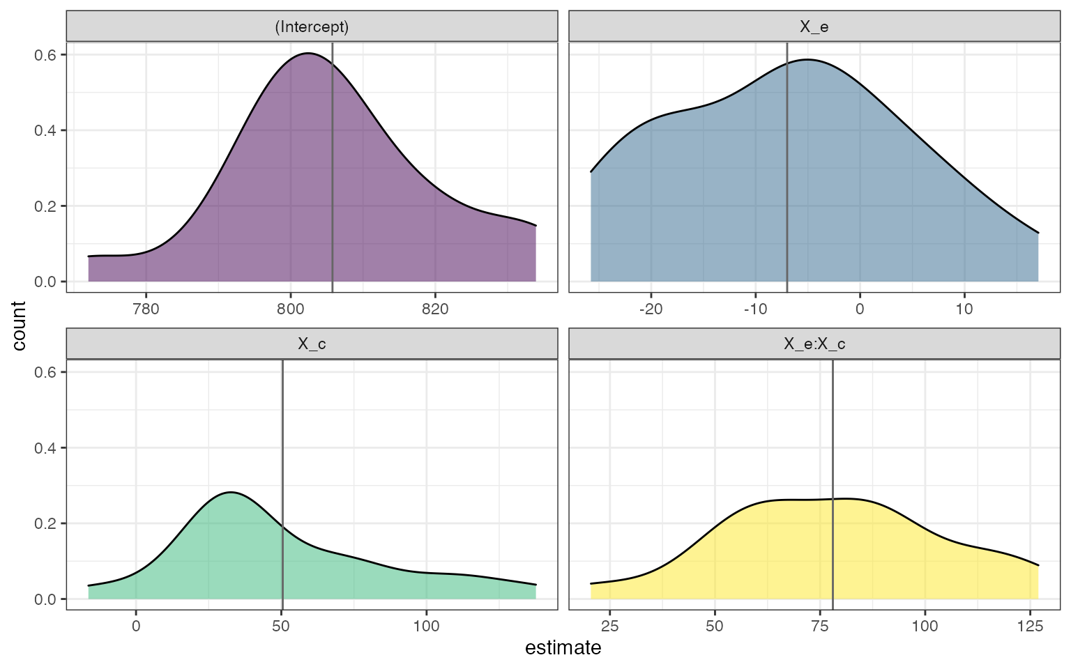
Distribution of fixed effects across simulations
sim_stats <- sims %>%
  filter(effect == "ran_pars") %>%
  group_by(group, term) %>%
  summarise(value = mean(estimate),
            .groups = "drop")

sims %>%
  filter(effect == "ran_pars") %>%
  ggplot(aes(estimate, fill = group)) +
  geom_density(alpha = 0.5, show.legend = FALSE) +
  geom_vline(data = sim_stats, aes(xintercept = value),
             show.legend = FALSE) +
  facet_wrap(~group*term, ncol = 3, scales = "free") +
  theme_bw()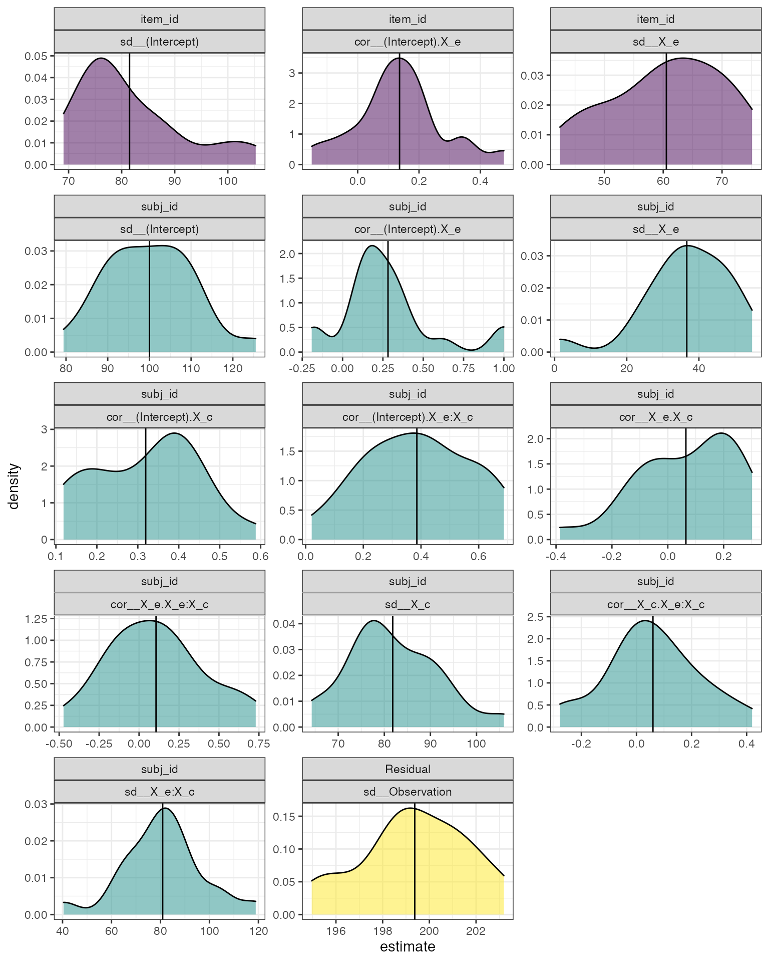
Distribution of random effects across simulations
2ww2ww Design with Counterbalancing
What if you change your design, and now category in a within-face factor, so each face can be either ingroup or outgroup. Subjects see each face only once in only one expression; whether a face is ingroup or outgroup, and happy or angry, is counterbalanced between subjects. Therefore, we need to change the data generating function a bit, although the rest of the code above doesn’t need to change.
Since category is now a within-subject factor, we need to add random slopes for category and the category*expression interaction for subjects, plus all of their correlations. We will also be specifying the subject and item Ns a little differently, as number of subjects per each of the 4 counterbalanced versions, and number of items per each of 4 groupsused in the counterbalancing.
# data simulation for a design with a 2x2 design where
# the first factor is within subjects and within items,
# and the second factor is within subjects and within items
# subjects see each face only once; whether a face is ingroup or outgraoup is counterbalanced between subjects

sim_data_2ww2ww <- function(
  n_subj     =  50, # number of subjects in each counterbalance group
  n_item     =  25, # number of items in each counterbalance group
  beta_0     = 800, # intercept (grand mean)
  beta_e     =  50, # main effect of category
  beta_c     =   0, # main effect of expression
  beta_ec    =  70, # interaction between category and expression
  subj_0     = 100, # by-subject random intercept sd
  subj_e     =  40, # by-subject random slope sd for exp
  subj_c     =  80, # by-subject random slope sd for category
  subj_ec    =  80, # by-subject random slope sd for category*exp
  # by-subject random effect correlations
  subj_rho   = c(.3, .3, .3,   # beta_0 * beta_c, beta_e, beta_ce
                     .1, .1,   # beta_c *         beta_e, beta_ce
                         .1),  # beta_e *                 beta_ce
  item_0     =  80, # by-item random intercept sd
  item_e     =  60, # by-item random slope for exp
  item_c     =  70, # by-item random slope sd for category
  item_ec    =  70, # by-item random slope sd for category*exp
  # by-item random effect correlations
  item_rho   = c(.2, .2, .2,   # beta_0 * beta_c, beta_e, beta_ce
                     .1, .1,   # beta_c *         beta_e, beta_ce
                         .1),  # beta_e *                 beta_ce
  sigma      = 200   # residual (error) sd
) {

  # simulate items
  items <- faux::rnorm_multi(
    n = n_item * 4,
    mu = 0,
    sd = c(item_0, item_e, item_c, item_ec),
    r = item_rho,
    varnames = c("I_0", "I_e", "I_c", "I_ec")
  ) %>%
    mutate(item_id = faux::make_id(nrow(.), "I"),
           # faces are in 1 of 4 groups
           grp_i = rep(1:4, n_item))

  # simulate subjects
  subjects <- faux::rnorm_multi(
    n = n_subj * 4,
    mu = 0,
    sd = c(subj_0, subj_e, subj_c, subj_ec),
    r = subj_rho,
    varnames = c("S_0", "S_e", "S_c", "S_ec")
  ) %>%
    mutate(subj_id = faux::make_id(nrow(.), "S"),
           # subjects view 1 of 4 counterbalanced versions
           cb = rep(LETTERS[1:4], n_subj))

  # simulate trials
  all_trials <- crossing(subjects, items,
    expression = factor(c("happy", "angry"), ordered = TRUE),
    category = factor(c("ingroup", "outgroup"), ordered = TRUE)
  )

  # keep only correct CB
  #     A   B   C   D
  # 1 = IH, IA, OH, OA
  # 2 = IA, IH, OA, OH
  # 3 = OH, OA, IH, IA
  # 4 = OA, OH, IA, IH
  trials <- filter(all_trials,
    (cb == "A" & grp_i == 1 & category == "ingroup" & expression == "happy") |
    (cb == "A" & grp_i == 2 & category == "ingroup" & expression == "angry") |
    (cb == "A" & grp_i == 3 & category == "outgroup" & expression == "happy") |
    (cb == "A" & grp_i == 4 & category == "outgroup" & expression == "angry") |
    (cb == "B" & grp_i == 2 & category == "ingroup" & expression == "happy") |
    (cb == "B" & grp_i == 1 & category == "ingroup" & expression == "angry") |
    (cb == "B" & grp_i == 4 & category == "outgroup" & expression == "happy") |
    (cb == "B" & grp_i == 3 & category == "outgroup" & expression == "angry") |
    (cb == "C" & grp_i == 3 & category == "ingroup" & expression == "happy") |
    (cb == "C" & grp_i == 4 & category == "ingroup" & expression == "angry") |
    (cb == "C" & grp_i == 1 & category == "outgroup" & expression == "happy") |
    (cb == "C" & grp_i == 2 & category == "outgroup" & expression == "angry") |
    (cb == "D" & grp_i == 4 & category == "ingroup" & expression == "happy") |
    (cb == "D" & grp_i == 3 & category == "ingroup" & expression == "angry") |
    (cb == "D" & grp_i == 2 & category == "outgroup" & expression == "happy") |
    (cb == "D" & grp_i == 1 & category == "outgroup" & expression == "angry"))

  trials %>%
    mutate(
      # effect code the two fixed factors
      X_e = recode(expression, "happy" = -0.5, "angry" = 0.5),
      X_c = recode(category, "ingroup" = -0.5, "outgroup" = +0.5),
      # add together fixed and random effects for each effect
      B_0  = beta_0  + S_0  + I_0,
      B_e  = beta_c  + S_e  + I_e,
      B_c  = beta_e  + S_c  + I_c,
      B_ec = beta_ec + S_ec + I_ec,
      # generate the error term
      e_si = rnorm(nrow(.), mean = 0, sd = sigma),
      # calculate RT by adding each effect term
      # multiplied by the relevant effect-coded factor(s)
      RT = B_0 + (B_e*X_e) + (B_c*X_c) + (B_ec*X_e*X_c) + e_si
    ) %>%
    select(subj_id, item_id, cb, expression, category, X_e, X_c, RT)
}
This is really tricky, so test your data thoroughly:
dat_sim <- sim_data_2ww2ww()

group_by(dat_sim, cb, expression, category) %>%
  summarise(n_subj = n_distinct(subj_id),
            n_item = n_distinct(item_id),
            mean_RT = mean(RT))
## # A tibble: 16 x 6
## # Groups: cb, expression [8]
## cb expression category n_subj n_item mean_RT
## <chr> <ord> <ord> <int> <int> <dbl>
## 1 A angry ingroup 50 25 750.
## 2 A angry outgroup 50 25 860.
## 3 A happy ingroup 50 25 764.
## 4 A happy outgroup 50 25 796.
## 5 B angry ingroup 50 25 726.
## 6 B angry outgroup 50 25 870.
## 7 B happy ingroup 50 25 805.
## 8 B happy outgroup 50 25 831.
## 9 C angry ingroup 50 25 801.
## 10 C angry outgroup 50 25 841.
## 11 C happy ingroup 50 25 799.
## 12 C happy outgroup 50 25 801.
## 13 D angry ingroup 50 25 782.
## 14 D angry outgroup 50 25 846.
## 15 D happy ingroup 50 25 841.
## 16 D happy outgroup 50 25 799.Analyse Data
The power function is similar to above, with a different data generating function and a different formula in the model.
# set up the power function
single_run2 <- function(filename = NULL, ...) {
  dat_sim <- sim_data_2ww2ww(...) # change to 2ww2ww version

  mod_sim <- lmer(RT ~ 1 + X_e*X_c +
                    (1 + X_e*X_c | item_id) + # add X_c here now it's w/in items
                    (1 + X_e*X_c | subj_id),
                  data = dat_sim)

  sim_results <- broom.mixed::tidy(mod_sim)

  # append the results to a file if filename is set
  if (!is.null(filename)) {
    append <- file.exists(filename) # append if the file exists
    write_csv(sim_results, filename, append = append)
  }

  # return the tidy table
  sim_results
}
Power Analysis
filename <- "sims/ext_sims_2.csv" # change for new analyses
if (!file.exists(filename)) {
  # run simulations and save to a file
  reps <- 20
  sims <- purrr::map_df(1:reps, ~single_run2(filename))
}

# read saved simulation data
sims <- read_csv(filename, col_types = cols(
  # makes sure plots display in this order
  group = col_factor(ordered = TRUE),
  term = col_factor(ordered = TRUE)
))