3  Historical

Setup

library(tidyverse)
library(showtext)

font_add(family = "Market Deco",
         regular = "fonts/Market_Deco.ttf")
font_add_google("Sen")
showtext_auto()

3.1 Population Data

I got this dataset from Our World in Data.

Code

pop <- read_csv("data/population-past-future.csv",
                show_col_types = FALSE)

spec(pop)

cols(
  Entity = col_character(),
  Code = col_character(),
  Year = col_double(),
  `Population (historical estimates and future projections)` = col_double()
)

The column names need some cleaning (I prefer to work with column names that are all lowercase with no spaces), and I don’t need some of the data.

Code

pop <- read_csv("data/population-past-future.csv",
                col_names = c("region", "year", "population"),
                skip = 1,
                col_types = "c-id")

head(pop)

region	year	population
Afghanistan	-10000	14737
Afghanistan	-9000	20405
Afghanistan	-8000	28253
Afghanistan	-7000	39120
Afghanistan	-6000	54166
Afghanistan	-5000	74999

3.2 Select relevant data

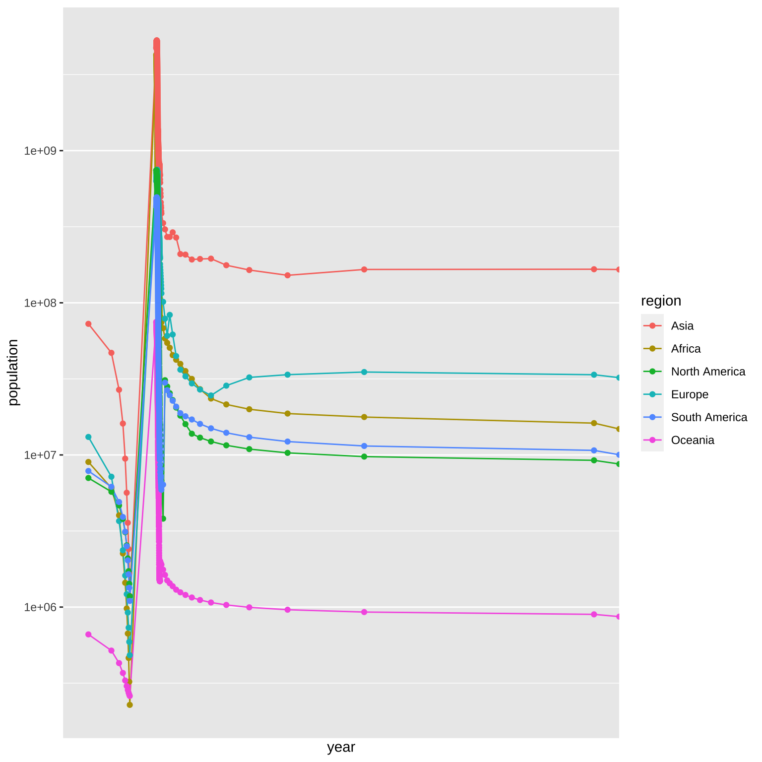
I just want to plot the population for the 6 major world regions, so I’ll filter that and make a quick line plot to see what I’ve got.

Code

world_regions <- pop %>%
  filter(region %in% c("Africa", "Asia", "Europe", "Oceania", "North America", "South America"))

Code

ggplot(world_regions, aes(x = year, y = population, color = region)) +
  geom_line()

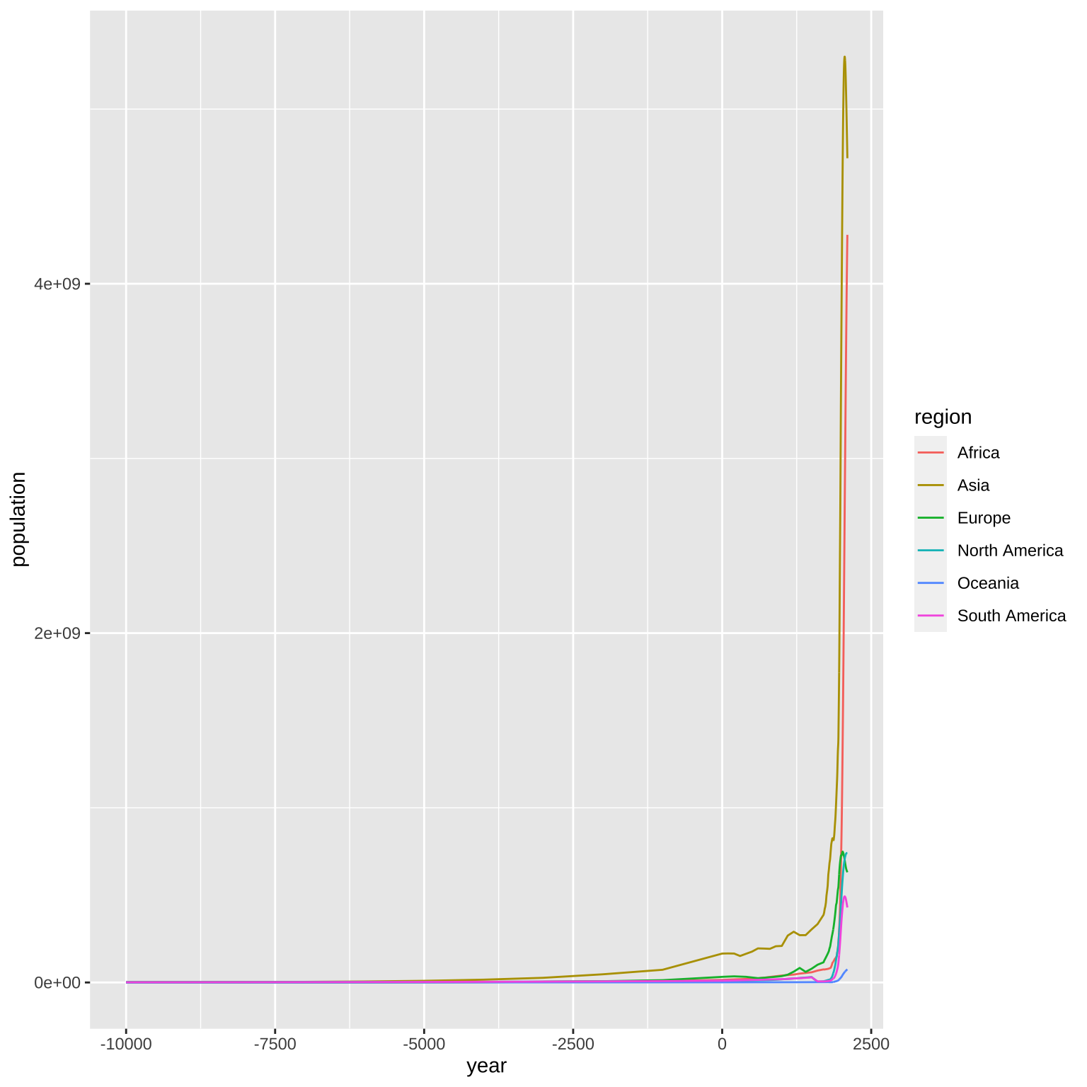
3.3 Transform y-axis

The population growth is pretty exponential at the end, so a log transformation of the y-axis might help.

Code

ggplot(world_regions, aes(x = year, y = population, color = region)) +
  geom_line() +
  scale_y_log10()

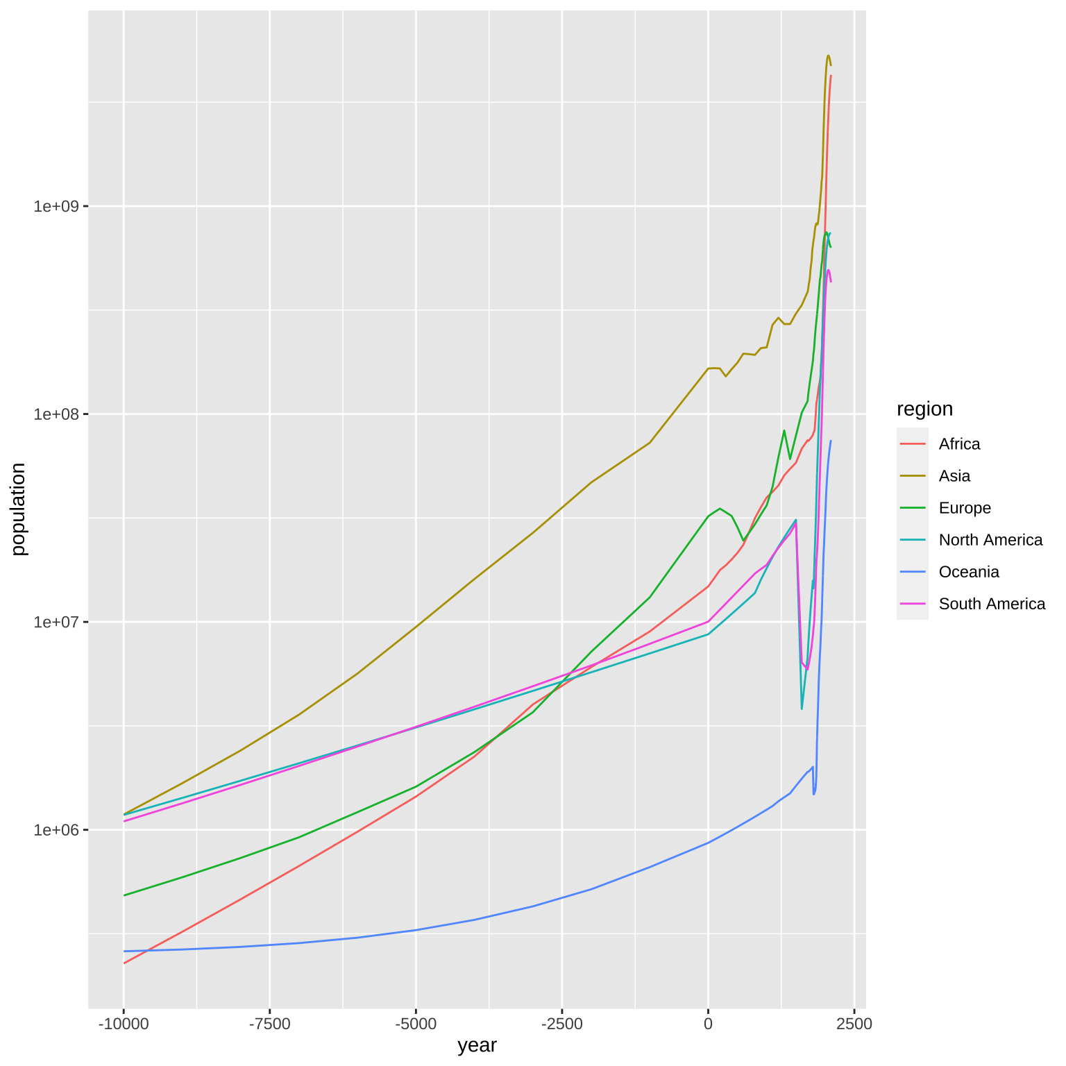
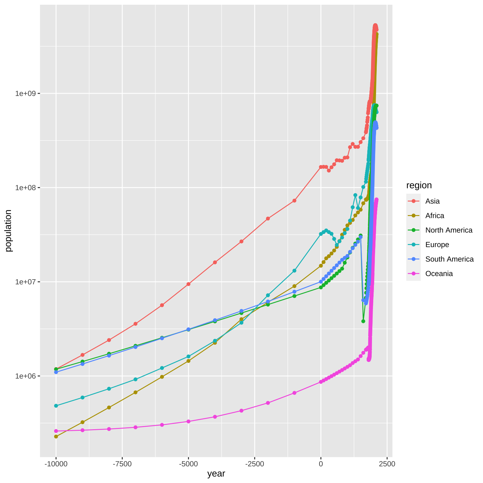
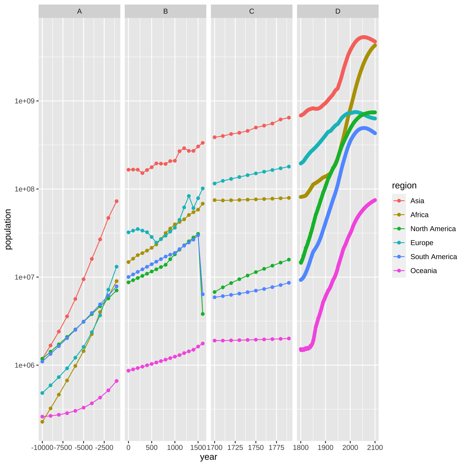
3.4 Region order

It would make more sense if the legend was in the same order as the lines, so I’ll turn that column into a factor ordered by the population at the latest year.

Code

region_order <- world_regions %>%
  filter(year == max(year)) %>%
  arrange(desc(population)) %>%
  pull(region)

world_regions <- world_regions %>%
  mutate(region = factor(region, region_order))

I’ll also add a point for each year with data.

Code

ggplot(world_regions, aes(x = year, y = population, color = region)) +
  geom_line() +
  geom_point() +
  scale_y_log10()

3.5 Variable x-axis

The data collection isn’t even at all. The years go every 1000 from -10000 to 0, then every 100 from 0 to 1700, then every 10 from 1700 to 1800, then every year from 1800 to 2021.

Code

unique(world_regions$year) %>% sort() %>% `[`(1:50)

 [1] -10000  -9000  -8000  -7000  -6000  -5000  -4000  -3000  -2000  -1000
[11]      0    100    200    300    400    500    600    700    800    900
[21]   1000   1100   1200   1300   1400   1500   1600   1700   1710   1720
[31]   1730   1740   1750   1760   1770   1780   1790   1800   1801   1802
[41]   1803   1804   1805   1806   1807   1808   1809   1810   1811   1812

I tried a few x-axis transformations, and they’re not straightforward because the x-axis crosses 0, which most transformations can’t handle. This was one of the silliest.

Code

ggplot(world_regions, aes(x = year, y = population, color = region)) +
  geom_line() +
  geom_point() +
  scale_y_log10() +
  scale_x_continuous(trans = "reciprocal")

So I’ll add a new column that specifies which time period they’re in. I’ll replace this text later, so it’s probably easiest to give them alphabetic labels now.

Code

world_regions <- world_regions %>%
  mutate(time_period = case_when(
      year < 0 ~ "A",
      year < 1700 ~ "B",
      year < 1800 ~ "C",
      year < 2101 ~ "D"))

Code

ggplot(world_regions, aes(x = year, y = population, color = region)) +
  geom_line() +
  geom_point() +
  scale_y_log10() +
  facet_grid(~time_period, scales = "free_x")

3.6 Clean Up

Now we’re getting somewhere, but still need to clean this up a lot. I’m going to remove the panel spacing and expansion so the plots touch each other. I’ll also customise the breaks and labels for the y-axis to make that easier to understand, and customise the colours (I do love a rainbow).

Code

# custom colours
rainbow <- c("#983E82","#E2A458","#F5DC70","#59935B","#467AAC","#61589C")

ggplot(world_regions, aes(x = year, y = population, color = region)) +
  geom_line() +
  geom_point() +
  facet_grid(~time_period, scales = "free_x") +
  scale_x_continuous(name = NULL,
                     expand = expansion(0)) +
  scale_y_log10(name = "Population (log scale)",
                breaks = 10^(5:10),
                labels = c("100K", "1M", "10M", "100M", "1B", "10B"),
                limit = c(1e5, 1e10)) +
  scale_color_manual(name = NULL,
                     values = rainbow) +
  theme_bw() +
  theme(axis.title.x = element_blank(),
        axis.text.x = element_text(angle = 90, hjust = 1),
        panel.spacing.x = unit(0, "cm"))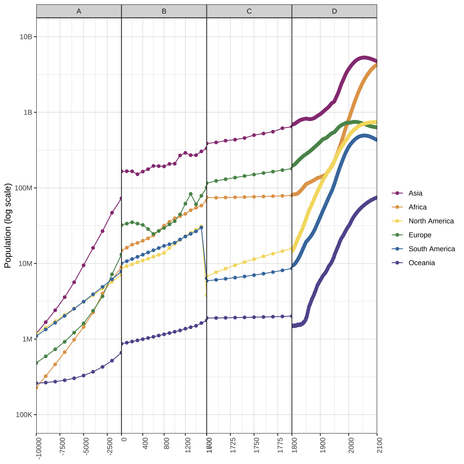

However, the borders of each time period don’t meet. I can fix that by duplicating the border years and assigning them to the previous time period.

Code

borders <- world_regions %>%
  group_by(time_period) %>%
  filter(year == min(year)) %>%
  ungroup() %>%
  filter(time_period != "A") %>%
  mutate(time_period = recode(time_period, B = "A", C = "B", D = "C"))

world_regions2 <- bind_rows(world_regions, borders)

Let’s also fix the facet labels. The function as_labeller() lets you translate between the data labels and custom labels for facets. And set some custom colours and custom x-axis breaks and labels. I moved the legend inside the plot to give the plot more horizontal room.

Code

# custom facet labels
tp_labels <- c(
  A = "10000BC to 0",
  B = "0 to 1700",
  C = "1700 to 1800",
  D = "1800 to 2100"
)

# custom x-axis breaks and labels
x_breaks <- c(seq(-10000, -2000, 2000),
              seq(0, 1600, 200),
              seq(1700, 1790, 10),
              seq(1800, 2100, 20))

x_labels <- c(paste(seq(10000, 2000, -2000), "BCE"),
              seq(0, 1700, 200),
              seq(1700, 1790, 10),
              seq(1800, 2100, 20))

ggplot(world_regions2, aes(x = year, y = population, color = region)) +
  geom_line() +
  geom_point() +
  facet_grid(~time_period, 
             scales = "free_x", 
             labeller = as_labeller(tp_labels)) +
  scale_x_continuous(name = NULL,
                   breaks = x_breaks,
                   labels = x_labels,
                   expand = expansion(0)) +
  scale_y_log10(name = "Population (log scale)",
                breaks = 10^(5:10),
                labels = c("100K", "1M", "10M", "100M", "1B", "10B"),
                limit = c(1e5, 1e10)) +
  scale_color_manual(name = NULL,
                     values = rainbow) +
  theme_bw() +
  theme(axis.text.x = element_text(angle = 90, hjust = 1),
        panel.spacing.x = unit(0, "cm"),
        legend.background = element_rect(fill = "transparent"),
        legend.position = c(.1, .75) )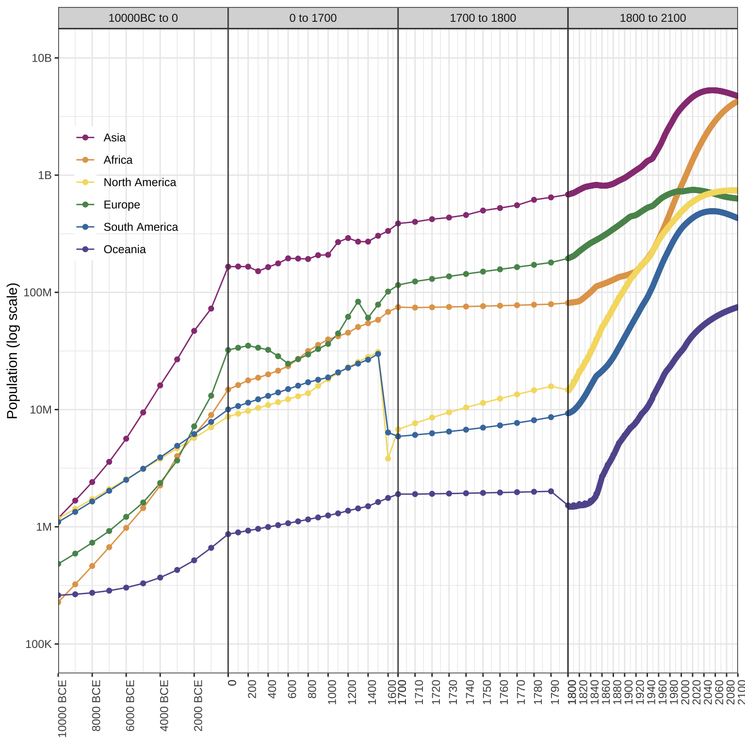

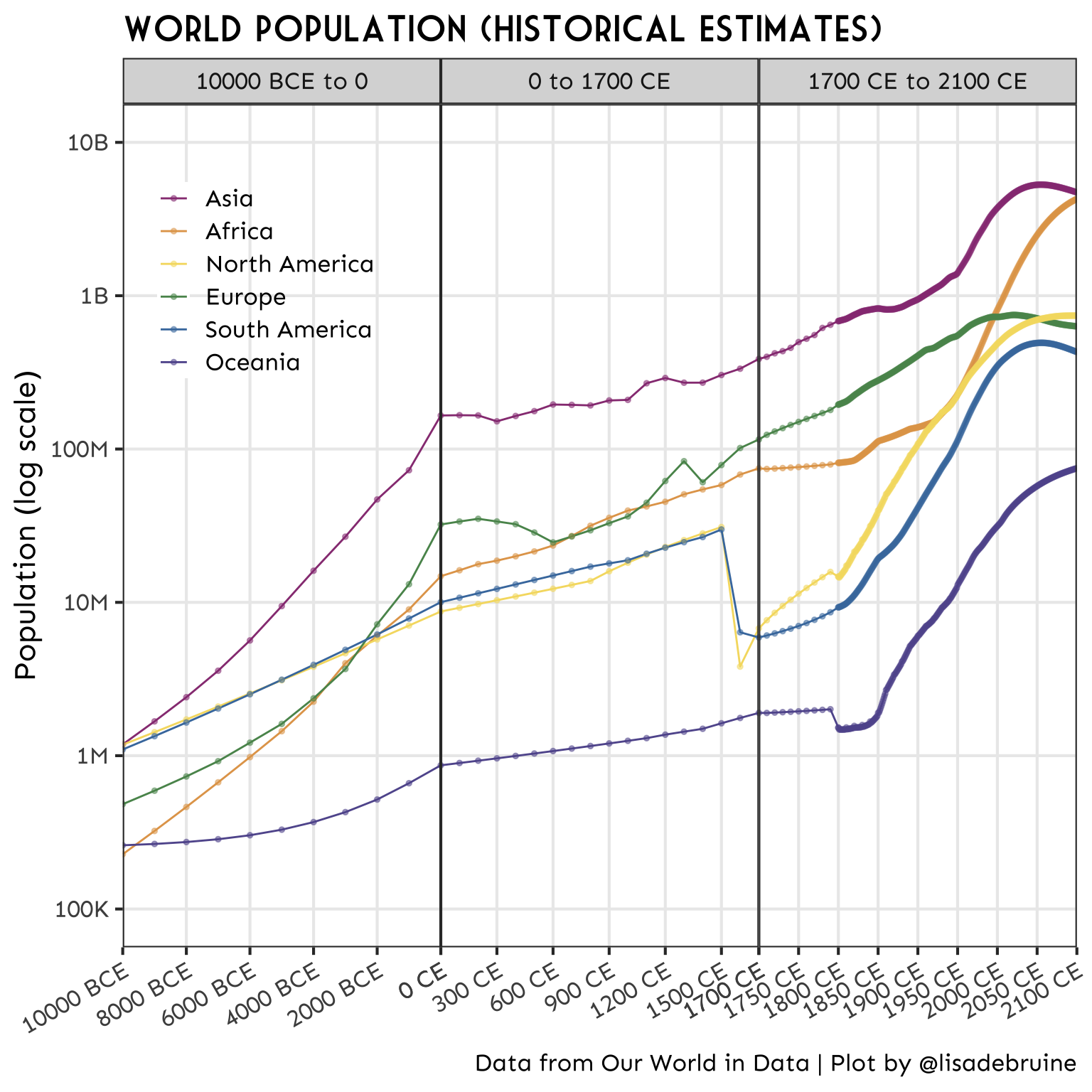
3.7 Change time periods

I changed by mind about 1700 to 1800. This plot gives it too much prominence. so I’ll combine it with 1800+. It looked weird to specify “BCE” only for the years before 0, so I added “CE” (Common Era) to the years after 0 and adjusted the angle and number of labels to make it easier to read.

Code

# recode time period to 3 periods (merge C and D)
world_regions3 <- world_regions2 %>%
  mutate(time_period = recode(time_period, A = "A", B = "B", C = "C", D = "C"))

# remake facet labels
tp_labels <- c(
  A = "10000 BCE to 0",
  B = "0 to 1700 CE",
  C = "1700 CE to 2100 CE"
)

# remake x-axis breaks and labels
x_breaks <- c(seq(-10000, -2000, 2000),
              seq(0, 1500, 300),
              seq(1700, 2100, 50))

x_labels <- c(paste(seq(10000, 2000, -2000), "BCE"),
              paste(seq(0, 1500, 300), "CE"),
              paste(seq(1700, 2100, 50), "CE"))

Code

ggplot(world_regions3, aes(x = year, y = population, color = region)) +
  geom_line() +
  geom_point(size = 1, alpha = 0.5) +
  facet_grid(~time_period, 
             scales = "free_x", 
             labeller = as_labeller(tp_labels)) +
  scale_x_continuous(name = NULL,
                   breaks = x_breaks,
                   labels = x_labels,
                   expand = expansion(0)) +
  scale_y_log10(name = "Population (log scale)",
                breaks = 10^(5:10),
                labels = c("100K", "1M", "10M", "100M", "1B", "10B"),
                limit = c(1e5, 1e10)) +
  scale_color_manual(name = NULL,
                     values = rainbow) +
  labs(title = "World Population (Historical Estimates)",
       caption = "Data from Our World in Data | Plot by @lisadebruine") +
  theme_bw(base_size = 16) +
  theme(text = element_text(family = "Sen"),
        axis.text.x = element_text(angle = 30, hjust = 1),
        panel.spacing.x = unit(0, "cm"),
        legend.background = element_rect(fill = "transparent"),
        legend.position = c(.15, .8),
        panel.grid.minor = element_blank(),
        plot.title = element_text(family = "Market Deco"))

World population estimates from 10000 BCE to 2021 CE.