23 Tiles
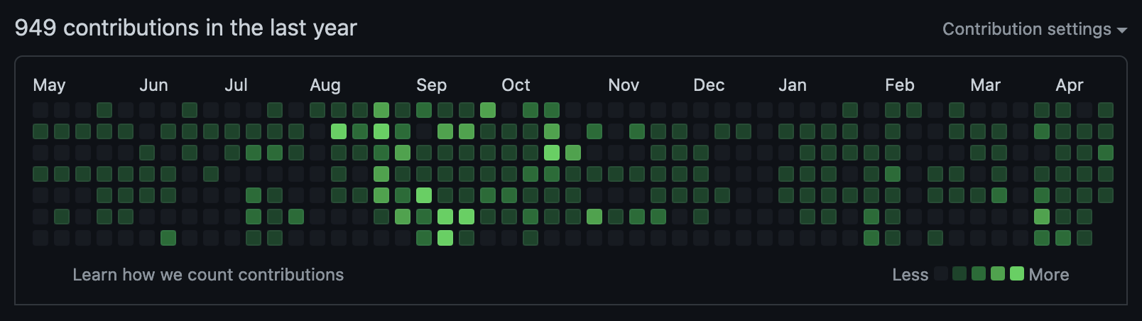
I really love the github activity tile graphs. For today’s plot, I’m going to use the methods from Day 21 the get data to make a similar plot, but showing all of the commits to repositories from the psyTeachR team.
Setup
library(httr)      # github authorisation
library(tidyverse) # for data wrangling
library(jsonlite)  # for reading JSON from GitHub API
library(glue)      # for text manipulation
library(lubridate) # for dates
library(scales)    # for axis scales
library(ggplotify) # for custom plot changes
library(showtext)  # for fonts

# install a good Scottish font
# https://www.fontspace.com/hill-house-font-f40002
font_add(family = "Hill House",
         regular = "fonts/Hill_House.otf")
showtext_auto()
23.1 Data
I need to use the GitHub API to get all the commit dates for the psyTeachR team. I followed a tutorial by Michael Galarnyk/ to set up the authorisation, since I’ll be making more than the maximum 60 requests per hour for unauthenticated users.
Set up OAuth
# Can be github, linkedin etc depending on application
oauth_endpoints("github")

# Change based on your app
myapp <- oauth_app(appname = "R_Code",
                   key = Sys.getenv("GITHUB_CLIENT_ID"),
                   secret = Sys.getenv("GITHUB_OAUTH_SECRET"))

# Get OAuth credentials
github_token <- oauth2.0_token(oauth_endpoints("github"), myapp)
gtoken <- config(token = github_token)
<oauth_endpoint>
authorize: https://github.com/login/oauth/authorize
access: https://github.com/login/oauth/access_token23.1.1 Get repo names
23.1.2 Forks
Most of the team work mainly in a fork on their own account and commit to the psyteachr origin rarely, so to get a clear picture of the work that the team does, we’ll also need to find all the forks.
I could get the members of the psyTeachR organisation through the GitHub API, but most haven’t made their membership public, thus only logged-in members can get this, so I’m just hard-coding their account names. We’ll use the psyteachr_forks list later.
Code
forks <- readRDS("data/forks.rds")

members <- c("BertlettJE", "carolinakt", "clelandwoods",
             "dalejbarr", "debruine", "eavanmac",
             "emilynordmann", "HelenaPaterson", "JackEdTaylor",
             "philmcaleer", "shannon-mcnee")

psyteachr_forks <- forks %>%
  select(full_name) %>%
  separate(full_name, c("user", "repo"), sep = "/") %>%
  filter(user %in% members)
23.1.3 Get commits
Get the commits for one repo first to see how they’re structured. I’ll choose the first ever psyTeachR group repo, called “R.House.2019”, which we made on a trip to Islay for a long weekend to learn git (and drink whisky) and actually did stay in an airBnB that was an R.House.

There’s a lot of data here, so let’s just extract the author, message and date for each commit.
Code
List of 3
 $ author : chr "debruine"
 $ message: chr "renamed files"
 $ date   : chr "2019-01-19T11:31:03Z"
23.1.4 Iterate
Now we just need to do this for every commit in every repository.
First, iterate over repos. You’re limited to 60 requests per hour without authenticating, which I don’t have time to figure out right now, so make sure you save this so you don’t lose it and set the code chunk to eval = FALSE or comment it out so you don’t accidentally run it again.
Code
# create API URLs for repos and forks
ptr_urls <- glue("https://api.github.com/repos/psyTeachR/{psyteachr_repos$name}/commits")
fork_urls <- glue("https://api.github.com/repos/{psyteachr_forks$user}/{psyteachr_forks$repo}/commits")
urls <- c(ptr_urls, fork_urls)

# get commit info for each repo
req <- map(urls, GET, gtoken)
psyteachr_commits <- map(req, parse_json, simplfyVector = TRUE)

# save to RDS object
saveRDS(psyteachr_commits, "data/psyteachr_commits.rds")
Iterate over all the repos and commits. Add columns with the date formatted as a date, year, week, and weekday.
Code
psyteachr_commits <- readRDS("data/psyteachr_commits.rds")

commit_info <- map_df(psyteachr_commits,
                   function(commits) {
    # iterate over commits for this repo
    map_df(commits, function(commit) {
      list(
        author = commit$commit$author$name,
        message = commit$commit$message,
        date = commit$commit$committer$date,
        url = gsub("(https\\://api\\.github\\.com/repos/|/commits/.*)", "", commit$url)
      )
    })%>%
        separate(url, c("user", "repo"), sep = "/")
  }) %>%
  # process versions of the date column
  mutate(date = lubridate::as_date(date),
         year = year(date),
         week = week(date),
         wday = wday(date))
23.2 Plot
23.2.1 Inital Plot
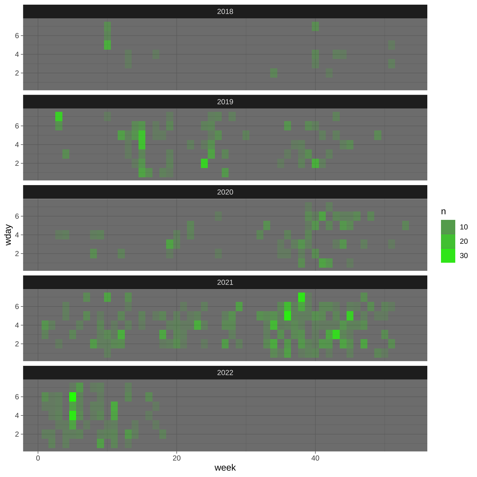
The first plot is usually pretty horrific, but this isn’t too bad.
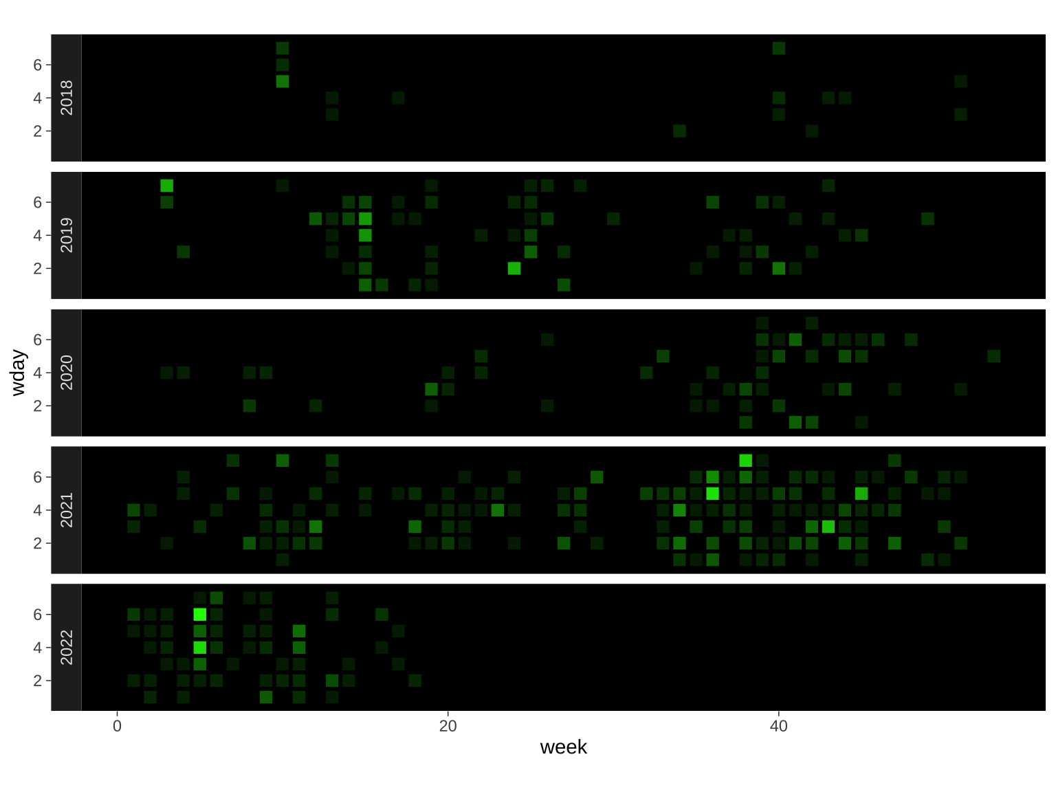
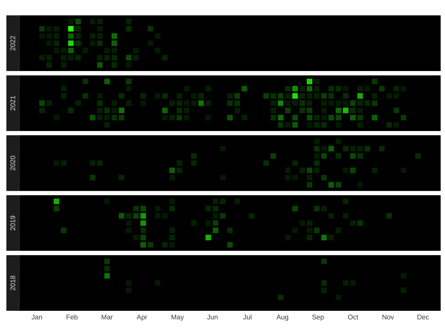
23.2.2 GitHub Theme
We can make this closer to the GitHub theme by fixing the coordinates so the tiles are square, making the panel backgrounds black, and getting rid of the grid lines. We can also free up a little more vertical space by putting the facet labels on the left. Add a black border to the tiles with size = 1.
Code
commits_by_day %>%
  ggplot(aes(x = week, y = wday, alpha = n)) +
  geom_tile(fill = "green", color = "black",
            size = 1, show.legend = FALSE) +
  facet_wrap(~year, ncol = 1, strip.position = "left") +
  coord_fixed() +
  theme_dark() +
  theme(
    panel.background = element_rect(fill = "black"),
    panel.grid = element_blank()
  )
23.2.3 Add months
The weeks of the year line up nicely, but don’t exactly correspond to months, so I’m going to hack this a little. I’ll add a secondary axis that rescales the weeks of the year to a 0.5 to 12.5 scale. The extra 0.5 is so the breaks can be set to 1:12 and the names of the month can go approximately in the middle of the month. I set position to “top” so the month axis would be on the bottom and I can hide the top axis (and some other parts we don’t need) using theme().
I also refactored year in the data so that 2022 displays at the top.
Code
commits_by_day$year <- factor(commits_by_day$year, levels = 2022:2018)

commits_by_day %>%
  ggplot(aes(x = week, y = wday, alpha = n)) +
  geom_tile(fill = "green", color = "black",
            size = 1, show.legend = FALSE) +
  scale_x_continuous(
    position = "top",
    sec.axis = sec_axis(
      trans = ~scales::rescale(., to = c(0.5, 12.5)),
      breaks = 1:12,
      labels = lubridate::month(1:12, T)
    )
  ) +
  facet_wrap(~year, ncol = 1, strip.position = "left") +
  labs(x = NULL, y = NULL) +
  coord_fixed() +
  theme_dark() +
  theme(
    panel.background = element_rect(fill = "black"),
    panel.grid = element_blank(),
    axis.ticks = element_blank(),
    axis.text.y = element_blank(),
    axis.text.x.top = element_blank()
  )
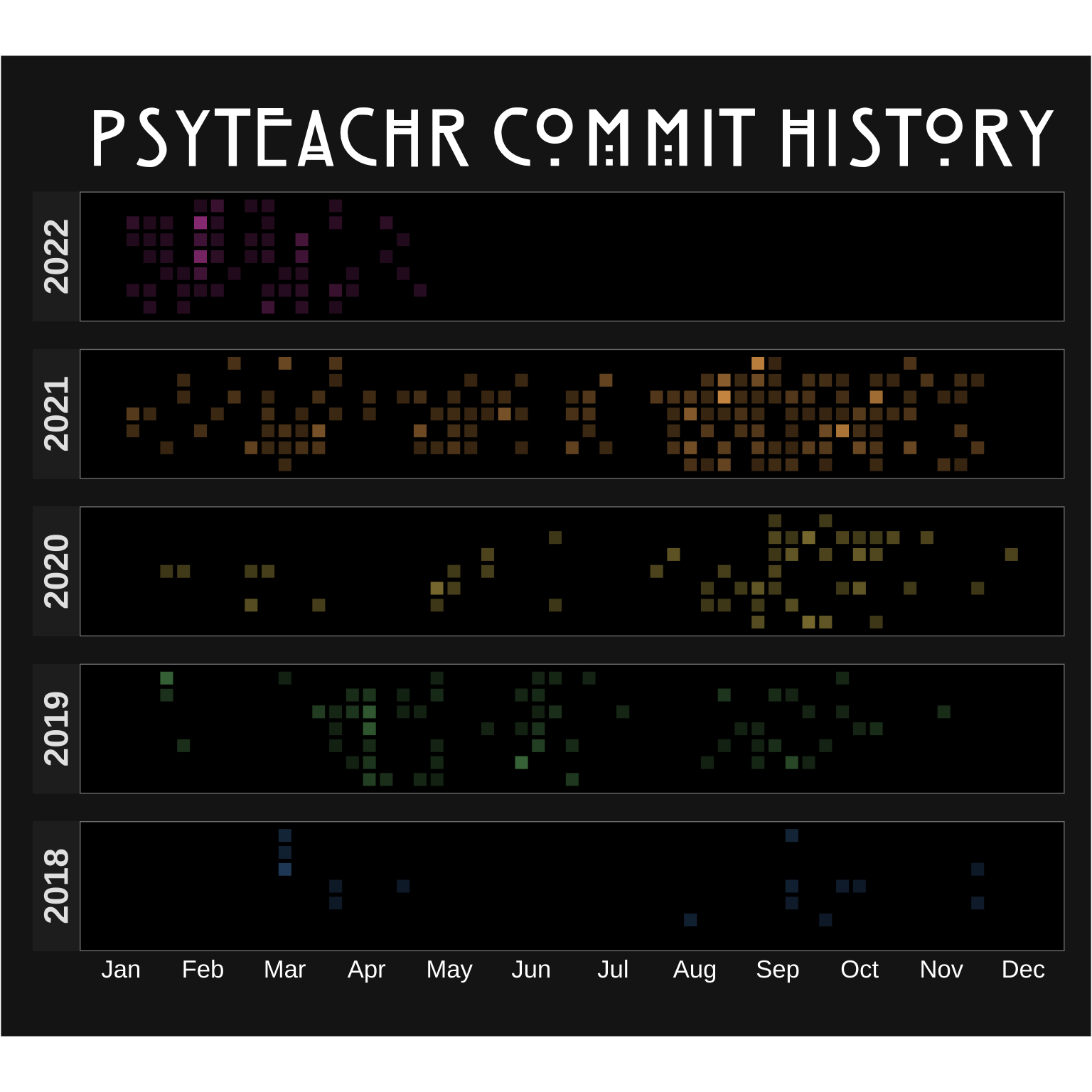
23.2.4 PsyTeachR Theme
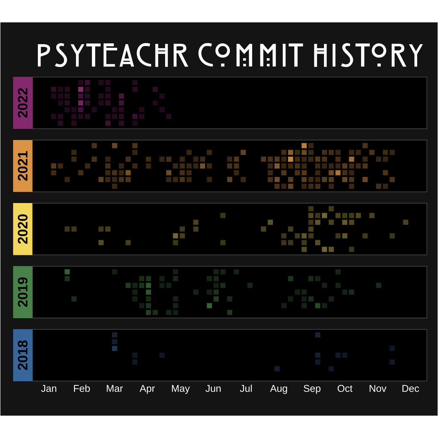
The psyTeachR books and website have a distinctive rainbow theme.

Set the fill to year and remove the green fill from geom_tile(). Use scale_fill_manual() to set the colours to the first 5 psyTeachR colours. Use scale_alpha() to set the minimum and maximum alpha values.
Code
commits_by_day %>%
  ggplot(aes(x = week, y = wday, alpha = n, fill = year)) +
  geom_tile(color = "black", size = 1, show.legend = FALSE) +
  scale_x_continuous(
    position = "top",
    sec.axis = sec_axis(
      trans = ~scales::rescale(., to = c(0.5, 12.5)),
      breaks = 1:12,
      labels = lubridate::month(1:12, T)
    )
  ) +
  scale_alpha(range = c(0.25, 1)) +
  scale_fill_manual(values = ptrc[1:5]) +
  facet_wrap(~year, ncol = 1, strip.position = "left") +
  labs(x = NULL, y = NULL, title = "PSYTEACHR COMMIT HISTORY") +
  coord_fixed() +
  theme_dark() +
  theme(
    plot.background = element_rect(fill = "grey10"),
    plot.margin = margin(2, 1, 2, 1, "lines"),
    panel.background = element_rect(fill = "black", color = "grey50"),
    panel.spacing = unit(1, "lines"),
    plot.title = element_text(family = "Hill House", size = 40, hjust = 0.5, color = "white"),
    strip.text = element_text(size = 18, face = "bold"),
    panel.grid = element_blank(),
    axis.ticks = element_blank(),
    axis.text.y = element_blank(),
    axis.text.x.top = element_blank(),
    axis.text.x.bottom = element_text(size = 13, color = "white")
  )
23.2.5 Change the facet strip color
I wanted to make the facet strip colour match the year’s tile colour, but it’s trickier than it sounds. I found this StackOverflow answer by utubun.
Code
p <- last_plot()
g <- ggplot_gtable(ggplot_build(p))
strips <- which(grepl('strip-', g$layout$name))

for (i in seq_along(strips)) {
  k <- which(grepl('rect', g$grobs[[strips[i]]]$grobs[[1]]$childrenOrder))
  l <- which(grepl('titleGrob', g$grobs[[strips[i]]]$grobs[[1]]$childrenOrder))
  g$grobs[[strips[i]]]$grobs[[1]]$children[[k]]$gp$fill <- ptrc[i]
  g$grobs[[strips[i]]]$grobs[[1]]$children[[l]]$children[[1]]$gp$col <- "black"
}
Now you can view the plot with plot(g) or convert it back to a ggplot object.