Appendix E — PsyArXiv

Setup

library(tidyverse) # for data wrangling
library(lubridate) # for handling dates
library(tidytext)  # for text analysis
library(ggraph)    # for plotting ngrams
library(magick)    # for cropping an image
library(grid)      # for raster

E.1 Data

PsyArXiv data from Day 27.

Code

preprint_data <- readRDS("data/preprint_data.RDS")

info <- map_df(preprint_data, function(p) {
  list(id = p$id,
       pub_dt = p$attributes$date_published,
       title = p$attributes$title,
       desc = p$attributes$description
       )
}) %>%
  mutate(pub_dt = as_datetime(pub_dt))

E.2 Ngrams

Here is a function that will extract any number of ngram.

Code

ngrams <- function(data, col, n = 2, sw = stop_words$word) {
  word_cols <- paste0("word_", 1:n)
  data %>%
    unnest_tokens(ngram, {{col}}, token = "ngrams", n = n) %>% 
    mutate(ngram_id = row_number()) %>%
    separate_rows(ngram, sep = " ") %>%
    filter(!ngram %in% sw) %>%
    group_by(ngram_id) %>%
    filter(n() == n) %>%
    mutate(word = word_cols) %>%
    ungroup() %>%
    pivot_wider(names_from = word, values_from = ngram) %>%
    count(across(all_of(word_cols)), sort = TRUE)
}

Look at the top 10 trigrams from a random 1000 entries.

Code

trigrams <- info %>%
  slice_sample(n = 1000) %>%
  ngrams(title, 3)

head(trigrams, 10)

word_1	word_2	word_3	n
covid	19	pandemic	24
randomized	controlled	trial	7
autism	spectrum	disorder	4
cross	lagged	panel	3
pilot	randomized	controlled	3
affective	task	switching	2
borderline	personality	disorder	2
cochlear	implant	listeners	2
cognitive	reflection	test	2
covid	19	lockdown	2

Calculate the bigrams for all titles.

Code

bigrams <- ngrams(info, title, 2)
head(bigrams, 10)

word_1	word_2	n
covid	19	1432
19	pandemic	549
mental	health	415
meta	analysis	406
systematic	review	302
individual	differences	217
social	media	125
emotion	regulation	108
virtual	reality	108
machine	learning	102

E.3 Plot

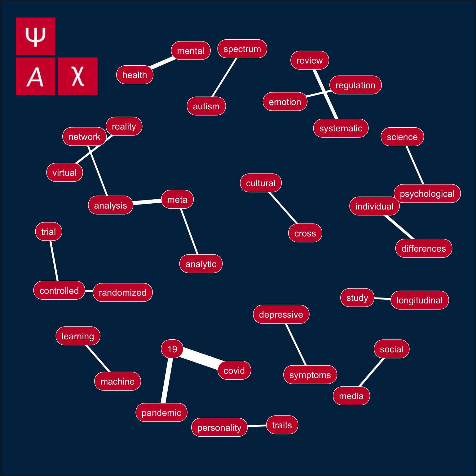
Use the code from Day 17 to make a bigram plot.

Code

bigrams %>%
  slice_max(order_by = n, n = 20) %>%
  ggraph(layout = "kk") +
  geom_edge_link(aes(width = n), color = "white", show.legend = FALSE) +
  geom_node_label(aes(label = name), vjust = 0.5, hjust = 0.5,
                  fill = "#CA1A31", color = "white", 
                  label.padding = unit(.5, "lines"),
                  label.r = unit(.75, "lines")) +
  coord_cartesian(clip = "off") +
  theme_void() +
  theme(plot.margin = unit(rep(.5, 4), "inches"),
        plot.background = element_rect(fill = "#012C4C"))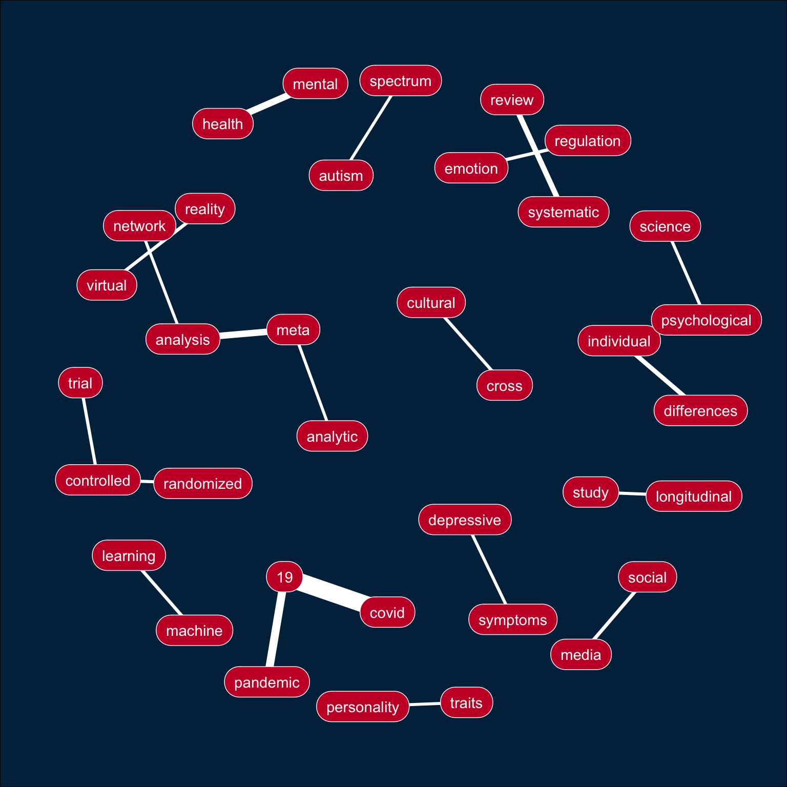

E.4 Add Image

Add the PsyArXiv logo using magick to crop the wikipedia logo and grid to rasterize it so it can be added as an annotation.

Process Image

#download.file("https://upload.wikimedia.org/wikipedia/commons/9/9c/PsyArXiv_logo.png", "images/psyarxiv.png")

# read and crop image
img <- magick::image_read("images/psyarxiv.png")
img_sq <- magick::image_crop(img, "174x174+4+4")
img_grob <- grid::rasterGrob(img_sq, interpolate=TRUE)

Plot Code

bigram_plot <- last_plot()

bigram_plot +
  annotation_custom(img_grob, 
                    xmin = -5, 
                    xmax =  -3, 
                    ymin = 1.2, 
                    ymax =  3.2)