7 Physical

Every time I thought about today’s prompt, by brain started playing Let’s Get Physical by Olivia Newton John. If you haven’t watched the video, it’s a real 80s experience. I’m going to try to theme the plot after the video.

I adapted some code from a tutorial I wrote on spotifyr, which is based on a tutorial by Michael Mullarkey. You can check those tutorials for the setup details if you haven’t used spotifyr before.

Setup

library(spotifyr)   # to access Spotify
library(tidyverse)  # for data wrangling

7.1 Get song ID

This step requires access to spotify and you can get timed out if you try to access it too much, so I always save the result of calls to an API in scripts and set that code chunk to eval = FALSE so it doesn’t run every time I render this book.

Code

# set to eval = FALSE to avoid too many call to spotify API
onj <- get_artist_audio_features(
  artist = 'Olivia Newton John',
  include_groups = "album"
)
saveRDS(onj, "data/onj.rds")

Now I can search the tracks for “Physical”. I’ll choose the earliest release.

Code

# read in saved object
onj <- readRDS("data/onj.rds")

physical_id <- onj %>%
  filter(track_name == "Physical") %>%
  filter(album_release_year == min(album_release_year)) %>%
  pull(track_id)

physical_id

[1] "273paQDMbi4JPeRfbYZuKx"

7.2 Song Analysis

Get the song analysis. It’s a list with a bunch of info.

Song analysis

# set to eval = FALSE to avoid too many call to spotify API
song_analysis <- get_track_audio_analysis(physical_id)
saveRDS(song_analysis, "data/song_analysis.rmd")

Read in saved object

# read in saved object
song_analysis <- readRDS("data/song_analysis.rmd")

meta gives you a list of some info about the analysis.
track gives you a list of attributes, including duration, loudness, end_of_fade_in, start_of_fade_out, and time_signature. Some of this info was available in the artist table.
bars, beats, and tatums are tables with the start, duration and confidence for each bar, beat, or tatum of music (whatever a “tatum” is).
sections is a table with the start, duration, loudness, tempo, key, mode, and time signature for each section of music, along with confidence measures of each.
segments is a table with information about loudness, pitch and timbre of segments of analysis, which tend to be around 0.2 seconds.

7.3 Pitches

The column pitches of the segments table has 12 values representing the degree of occurrence for each note in each time segment, so we have to unpack this a bit.

Pitch analysis

pitch_analysis <- song_analysis$segments %>%
  unnest(pitches) %>%
  rename(pitch_degree = pitches) %>%
  group_by(start) %>%
  mutate(pitch = row_number()-1) %>%
  ungroup() %>%
  filter(pitch_degree == 1) %>%
  select(start, duration, loudness_start, pitch)

head(pitch_analysis)

start	duration	loudness_start	pitch
0.000	0.488	-28.812	9
0.488	0.359	-25.662	9
0.847	0.204	-24.822	8
1.051	0.256	-24.402	1
1.307	0.573	-21.224	8
1.880	0.483	-23.087	9

Now I want to figure out the main pitch for each beat, so I need to somehow map the pitch table to the beat table. First, I need to work out the main segment in each beat.

Main pitch for each beat

seg <- song_analysis$segments %>%
  select(seg_start = start, seg_dur = duration)

beat <- song_analysis$beats %>%
  select(beat_start = start, beat_dur = duration)

main_seg_in_beat <- inner_join(seg, beat, by = character()) %>%
  mutate(seg_end = seg_start + seg_dur, 
         beat_end = beat_start + beat_dur,
         seg_in_beat = (seg_start <= beat_end) & (seg_end >= beat_start)) %>%
  filter(seg_in_beat) %>%
  rowwise() %>%
  mutate(overlap = min(seg_end, beat_end) - max(c(seg_start, beat_start)),
         pcnt_in_beat = overlap/beat_dur) %>%
  group_by(beat_start) %>%
  slice_max(order_by = pcnt_in_beat, n = 1) %>%
  ungroup()

head(main_seg_in_beat)

seg_start	seg_dur	beat_start	beat_dur	seg_end	beat_end	seg_in_beat	overlap	pcnt_in_beat
0.488	0.359	0.504	0.460	0.847	0.964	TRUE	0.344	0.747
1.051	0.256	0.964	0.473	1.307	1.437	TRUE	0.256	0.541
1.307	0.573	1.437	0.474	1.880	1.910	TRUE	0.443	0.936
1.880	0.483	1.910	0.469	2.363	2.380	TRUE	0.452	0.964
2.363	0.465	2.380	0.469	2.827	2.849	TRUE	0.448	0.954
2.827	0.446	2.849	0.474	3.274	3.322	TRUE	0.425	0.897

And then join this with the pitch analysis table to get a main pitch for each beat.

Pitch by beat

pitch_by_beat <- main_seg_in_beat %>%
  select(start = seg_start) %>%
  left_join(pitch_analysis, "start")

head(pitch_by_beat)

start	duration	loudness_start	pitch
0.488	0.359	-25.662	9
1.051	0.256	-24.402	1
1.307	0.573	-21.224	8
1.880	0.483	-23.087	9
2.363	0.465	-15.020	11
2.827	0.446	-21.016	0

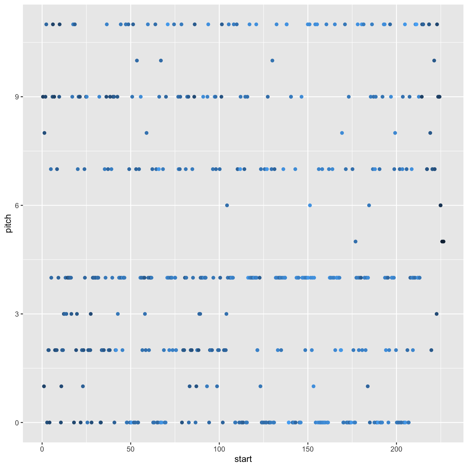
7.4 Plot Pitch by Beat

Code

ggplot(pitch_by_beat,
       aes(x = start, y = pitch, color = loudness_start)) +
  geom_point(show.legend = FALSE)

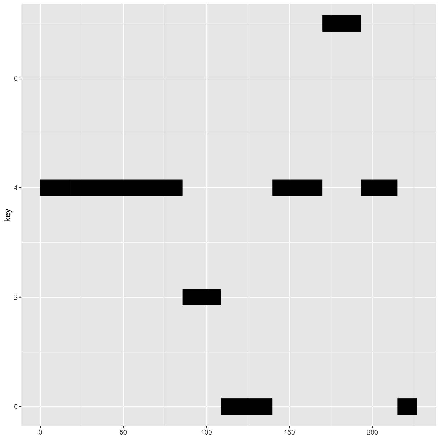
7.5 Plot Key by Segment

I also wanted to map the key of each segment using a horizontal linerange, so I mapped it vertically first and flipped the coordinates.

Code

ggplot(song_analysis$sections, aes(ymin = start, 
                               ymax = start + duration,
                               x = key)) +
  geom_linerange(size = 10) +
  coord_flip()

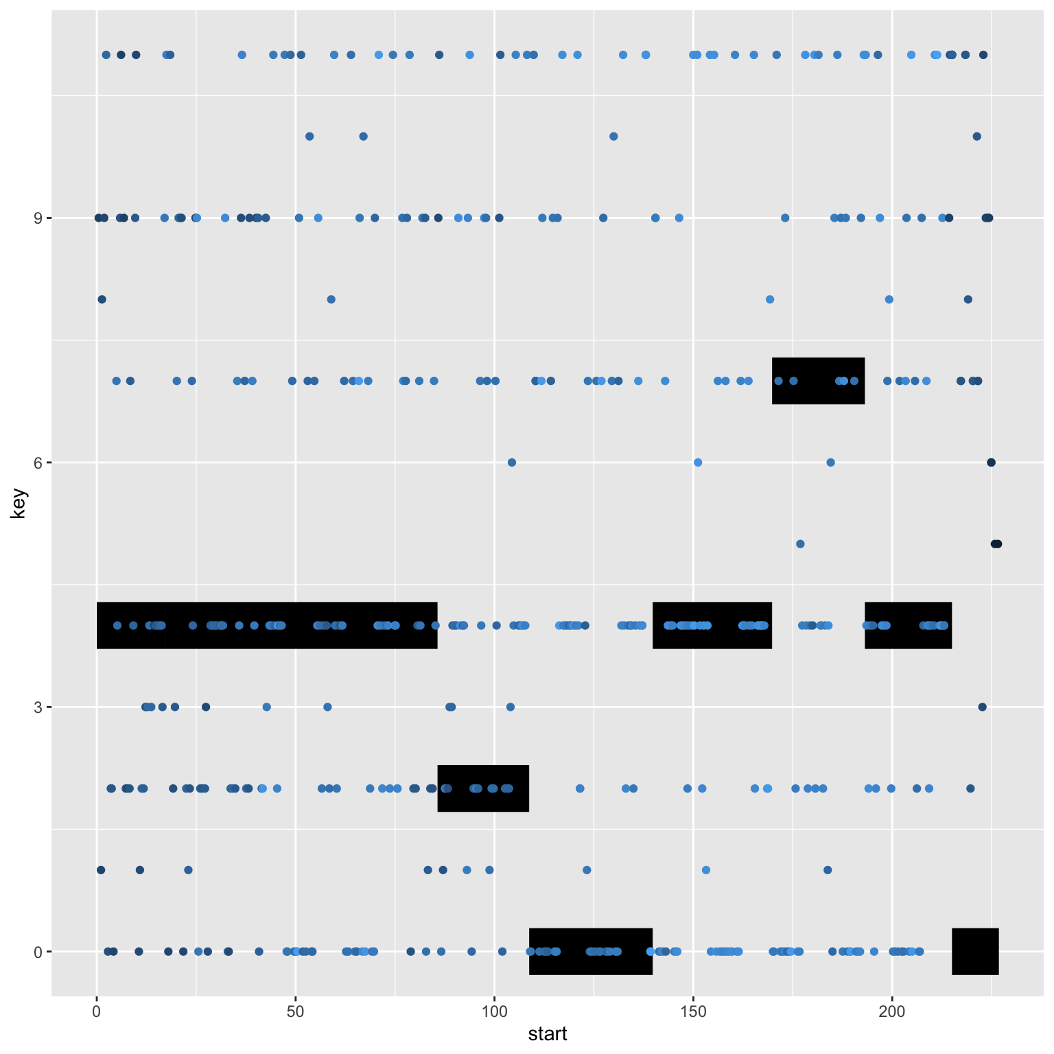
7.6 Combine Plots

So to combine them, I need to move the data and mapping to the relevant geoms and swap the x and y coordinates for the pitch points.

Code

ggplot() +
  geom_linerange(mapping = aes(ymin = start, 
                               ymax = start + duration,
                               x = key),
                 data = song_analysis$sections,
                 size = 12) +
  coord_flip() +
  geom_point(mapping = aes(y = start, x = pitch, color = loudness_start),
             data = pitch_by_beat, show.legend = FALSE)

7.7 80s Theme

Let’s remind ourselves of this monstrosity.

Code

# translate spotify's 0-11 to notes
pitch_key_vals <- c('C', 'C#/Db', 'D', 'D#/Eb', 'E', 'F', 
                     'F#/Gb', 'G', 'G#/Ab', 'A', 'A#/Bb', 'B')

ggplot() +
  geom_linerange(mapping = aes(ymin = start, 
                               ymax = start + duration,
                               x = key),
                 data = song_analysis$sections,
                 size = 12,
                 color = "#60E1FE") +
  coord_flip() +
  geom_point(mapping = aes(y = start, x = pitch, alpha = loudness_start),
             data = pitch_by_beat, 
             color = "#BB1DA8", size = 3,
             show.legend = FALSE) +
  scale_y_continuous(breaks = seq(0, 250, 20)) +
  scale_x_continuous(breaks = 0:11,
                     labels = pitch_key_vals) +
  scale_alpha(range = c(0, .6)) +
  labs(x = "Key/Pitch",
       y = NULL,
       title = "Let's Get Physical — Olivia Newton John",
       subtitle = "Main pitch for each beat (in pink) and key for each segment (in blue)",
       caption = "Data from Spotify via spotifyr | plot by @lisadebruine")  +
  theme_bw(base_size = 16) +
  theme(plot.subtitle = element_text(color = "red"),
        panel.background = element_rect(fill = "#091131"),
        panel.grid.major.y = element_blank(),
        panel.grid.minor.x = element_blank())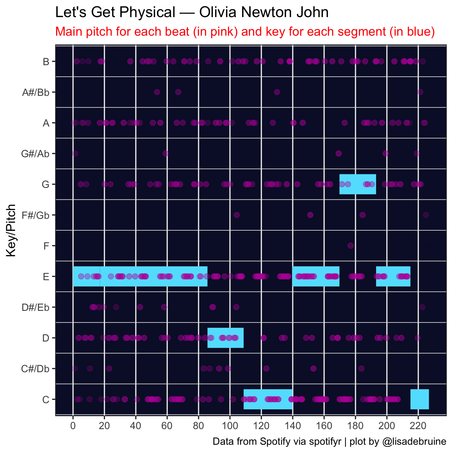

OK, that’s awful and I’m sorry. {fig-align=‘center’ fig-alt=‘Chart of Let’s Get Physical by Olivia Newton John, showing the main pitch for each beat (in pink) and key for each segment (in blue). The 80s visual theme is reminiscent of the gym from the music video for the song.’ width=100%}