13  Correlation

I’m a sucker for a silly correlation, and I’ve also been meaning to try out the ravelRy package for working with the ravelry API.

Setup

library(tidyverse) # for data wrangling
library(ravelRy)   # for searching ravelry 
library(rvest)     # for web scraping
library(DT)        # for interactive table
library(showtext)  # for fonts

# add the font Ravelry uses on their webpage
font_add_google(name = "Jost", family = "Jost")
showtext_auto()

# increase penalty for scientific notation
options(scipen = 4)

13.1 Craft Shops

I wanted to find the country of all the users on Ravelry, but the ravelRy package doesn’t have a function for searching people and I don’t have time to write one today, so I just searched for yarn shops, which also have a country attribute.

The slowly() function below is from purrr and retrieves 1000 yarn shops’ details every 10 seconds. There turned out to be 8072. You get an error if you try to retrieve an empty page of shops, so I wrapped the search_shops() code in tryCatch() so the function didn’t fail then. I saved the result to RDS so I can set this code chunk to eval = FALSE and read this in without calling the ravelry API every time I knit this book.

Code

slow_shop <- slowly(function(page) { 
  tryCatch({
    shops <- search_shops(page_size = 1000, page = page) 
    shops$country.name
  }, error = function(e) {})
}, rate = rate_delay(10))

shops <- map(1:10, slow_shop) %>% unlist()
saveRDS(shops, "data/yarn_shops.rds")

I had to fix some country names so they match with the other data sets. There is only one happiness value for the UK, so I reluctantly combined the four countries in the UK.

Code

shops <- readRDS("data/yarn_shops.rds")

shop_countries <- tibble(
  country = shops
) %>%
  mutate(country = recode(country,
                          Wales = "United Kingdom", 
                          Scotland = "United Kingdom",
                          England = "United Kingdom",
                          "Northern Ireland" = "United Kingdom",
                          "Viet Nam" = "Vietnam",
                          "Bosnia and Herzegowina" = "Bosnia and Herzegovina",
                          "Korea, Republic of" = "South Korea",
                          .default = country)) %>%
  count(country, name = "yarn_shops")

13.2 Temperature

I feel like average temperature might have something to do with the number of yarn shops in a country, so I scraped that from a Wikipedia page using rvest. I had to edit the Wikipedia page first because the table formatting was borked. I also had to fix the html minus symbol because it made the negative numbers read in as character strings.

Code

temp <- read_html("https://en.wikipedia.org/wiki/List_of_countries_by_average_yearly_temperature") %>%
  html_nodes('table.wikitable') %>%
  html_table(header = TRUE) %>%
  bind_rows() %>%
  as_tibble() %>%
  rename(country = 1, temp = 2) %>%
  mutate(temp = gsub("−", "-", temp)) %>%
  type_convert(col_types = "cd")

head(temp)

country	temp
Burkina Faso	NA
Mali	28.25
Kiribati	28.20
Djibouti	28.00
Maldives	28.00
Senegal	27.85

Then I decided maybe the average temperature for the coldest month was better, which I found on a site with the rather upsetting name listfist, but had problems reading it with rvest so gave up.

Code

html <- read_html("https://listfist.com/list-of-countries-by-average-temperature")

13.3 Happiness

I got the happiness ratings from the World Happiness Report, which also included a population column in units of thousands.

Code

happy <- read_csv("data/happiness_2022.csv",
                  show_col_types = FALSE) %>%
  mutate(pop2022 = pop2022 * 1000)

13.4 Join Data

Now to join all the data together.

Code

happy_craft <- shop_countries %>%
  left_join(happy, by = "country") %>%
  filter(!is.na(pop2022)) %>%
  left_join(temp, by = "country") %>%
  mutate(shops_per_M = 1e6 * yarn_shops / pop2022)

In case you want to find your country in the data.

Code

happy_craft %>%
  mutate(shops_per_M = round(shops_per_M, 3)) %>%
  select("Country" = country, 
         "Yarn Shops" = yarn_shops, 
         "Shops/M" = shops_per_M,
         Happiness = happiness2021, 
         Population = pop2022, 
         "Mean Temp" = temp) %>%
  DT::datatable()

13.5 Correlations

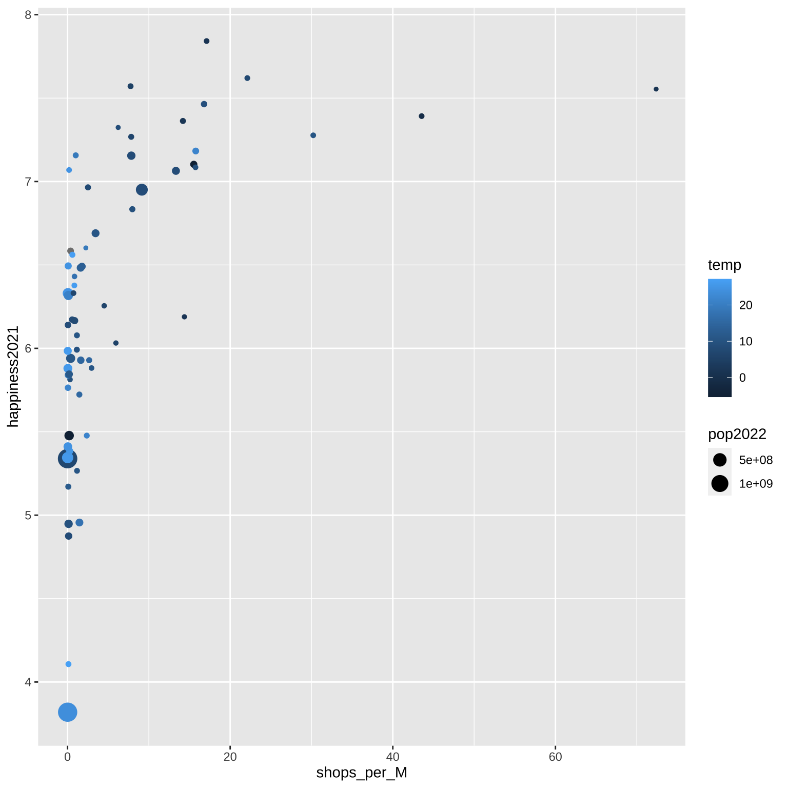
Let’s just have a quick look at the correlations here. The number of yarn shops per million population is positively correlated with happiness and negatively correlated with mean annual temperature. However, temperature is also negatively correlated with happiness.

Code

happy_craft %>%
  select(shops_per_M, happiness2021, temp) %>%
  cor(use = "pairwise.complete.obs") %>%
  round(2)

              shops_per_M happiness2021  temp
shops_per_M          1.00          0.55 -0.45
happiness2021        0.55          1.00 -0.39
temp                -0.45         -0.39  1.00

13.6 Initial Plot

First, I made a simple plot of the correlation between the number of yarn shops per million people and happiness score for each country. I set the size of the points relative to the population and the colour relative to the mean annual temperature.

Code

ggplot(happy_craft, aes(x = shops_per_M, 
                        y = happiness2021, 
                        size = pop2022,
                        color = temp)) +
  geom_point()

13.7 Customise the plot

Iceland is the outlier, with 72.4 yarn shops on Ravelry, so I’ll set the x-axis to log10. I’ll also use some annotations tricks I learned for Day 12.

Code

ggplot(happy_craft, aes(x = shops_per_M, 
                        y = happiness2021, 
                        size = pop2022,
                        color = temp)) +
  geom_smooth(mapping = aes(weight = pop2022),
              method = lm, formula = y~x, 
              color = "grey", alpha = 0.1,
              show.legend = FALSE) +
  geom_point() +
  
  # label a few countries
  annotate("text", label = "Iceland", color = "#404763", 
           hjust = 1, vjust = 1,
           x = 80, y = 7, size = 4) +
  annotate(geom = "curve", curvature = 0.3, size = 0.25,
            x = 80, y = 7, 
            xend = 73, yend = 7.5,
            arrow = arrow(length = unit(0.4, "lines"))) +
  annotate("text", label = "India", color = "#EF6E62", 
           hjust = 0, vjust = 0.5,
           x = .03, y = 4.1, size = 4) +
  annotate(geom = "curve", curvature = 0.3, size = 0.25,
            x = .03, y = 4.1, 
            xend = .017, yend = 4,
            arrow = arrow(length = unit(0.4, "lines"))) +
  annotate("text", label = "UK", color = "#94616C", 
           hjust = 1, vjust = 0.5,
           x = 8, y = 8.2, size = 4) +
  annotate(geom = "curve", curvature = -0.2, size = 0.25,
            x = 8, y = 8.2, 
            xend = 13, yend = 7.164,
            arrow = arrow(length = unit(0.4, "lines"))) +
  
  # scale functions
  scale_size_area("Population",
                  max_size = 10,
                  breaks = 10^(5:9),
                  labels = c("100K", "1M", "10M", "100M", "1B")) +
  scale_color_gradient("Mean Annual\nTemperature\n",
                       low = "#404763", high = "#EF6E62") +
  scale_y_continuous("Happiness Score (2021)",
                     limits = c(3.5, 8.5)) +
  scale_x_log10("Number of Yarn Shops on Ravelry per Million Population") +
  guides(size = "none") +
  labs(title = "Do Yarn Shops Cause Happiness?",
       subtitle = "Data from Ravelry, Wikipedia & World Happiness Report | Plot by @lisadebruine") +
  theme_classic(base_family = "Jost", base_size = 14) +
  theme(
    plot.title = element_text(face = "bold", color = "#EF6E62", size = 20),
    plot.subtitle = element_text(face = "italic", color = "#404763"),
    legend.position = c(.65, .12),
    legend.key.width = unit(.07, "npc"),
    legend.direction = "horizontal",
    legend.background = element_blank()
  )