18  OECD

I have a potential thesis student who wants to work with topic modelling next year. Although I have a publication using latent dirichtlet analysis (LDA), my former postdoc, Ant Lee, did the main analysis, so I need to brush up. I’m also keen to practice my web scraping skills, so I thought I’d scrape the OECD data insights page to see what topics they’ve been posting about.

Setup

library(tidyverse)   # for data wrangling
library(rvest)       # for web scraping
library(tidytext)    # for text analysis
library(topicmodels) # for topic modelling
library(MetBrewer)   # for beautiful colourblind-friendly colour schemes

theme_set(theme_minimal(base_size = 16))

18.1 Data

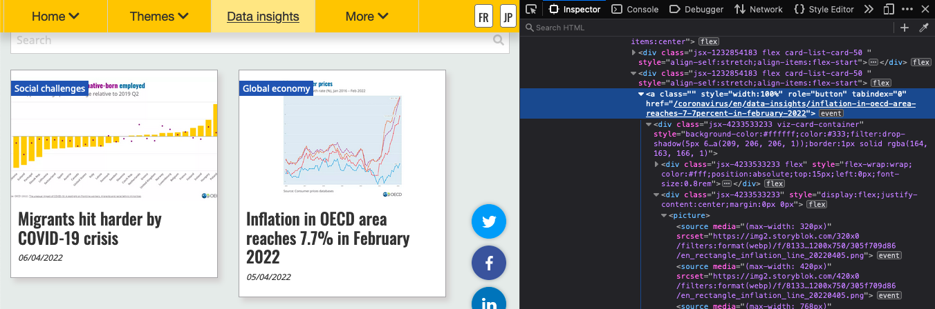
The data insights page only shows a few entries at first. So I had to click on “Show more” a bunch of times until I accessed all of them, and download the webpage first, then search the download with rvest.

I used the developer tools in FireFox to find out that each “card” had a class of “card-list-card-50” and the link to the insight page was in the only “a” tag in each card.

Figuring out the right nodes to search to scrape all the URLs.

Scrape URLS

# saved from https://www.oecd.org/coronavirus/en/data-insights/
html <- read_html("data/OECD | Data insights.html")
nodes <- html_nodes(html, ".card-list-card-50 a")
urls <- html_attr(nodes, "href")

# narrow down to only links to the data-insights section
insight <- map_lgl(urls, str_detect, "/data-insights/")
insight_urls <- urls[insight] %>% unique()

Then scrape the contents of each link and extract all of the paragraph text. Save this as a RDS object, set the code chunk to eval = FALSE, and load from that so this doesn’t scrape OECD every time.

Scrape paragraphs

p <- map_df(insight_urls, function(x) {
  read_html(x) %>%
    html_nodes("p") %>%
    html_text() %>%
    data.frame(url = x, p = .)
})

saveRDS(p, "data/oecd_covid_insights.rds")

Get rid of the rows that just have the text, “Follow us (Social Media):”.

Read previously scraped data

p <- readRDS("data/oecd_covid_insights.rds") %>%
  filter(p != "Follow us (Social Media):")

18.2 Topic Modelling

Now the fun part. I used the Topic Modelling chapter from Text Mining with R.

Code

words <- p %>%
  unnest_tokens(word, p)

# find document-word counts
word_counts <- words %>%
  anti_join(stop_words, by = "word") %>%
  count(word, sort = TRUE)

head(word_counts, 50) %>% pull(word)

 [1] "countries"     "oecd"          "covid"         "19"           
 [5] "economic"      "pandemic"      "2020"          "2021"         
 [9] "global"        "growth"        "economies"     "people"       
[13] "recovery"      "trade"         "crisis"        "outlook"      
[17] "health"        "measures"      "inflation"     "compared"     
[21] "sectors"       "women"         "energy"        "income"       
[25] "percentage"    "policy"        "food"          "economy"      
[29] "governments"   "green"         "support"       "data"         
[33] "expected"      "rates"         "digital"       "international"
[37] "levels"        "employment"    "tax"           "jobs"         
[41] "lower"         "world"         "2019"          "gdp"          
[45] "impact"        "pre"           "vaccines"      "supply"       
[49] "unemployment"  "united"       

Let’s get rid of all the integers 0 to 2030, “countries”, and “oecd”, which are likely to be so common as to be meaningless.

Code

sw <- data.frame(word = c(stop_words$word, 0:2030, "oecd", "countries"))

word_counts <- words %>%
  anti_join(sw, by = "word") %>%
  count(url, word, sort = TRUE)

18.2.1 LDA

Convert the word_counts table to dtm format and run the LDA. I used k = 6 to extract 6 topics. I tried a few different values with the interpretive steps below, and 6 seemed reasonable to interpret. There are formal ways to assess this, but it’s beyond what I have time to do today.

Code

# document term matrix
lda <- word_counts %>%
  cast_dtm(document = url, term = word, value = n) %>%
  LDA(k = 6, control = list(seed = 8675309))

18.2.2 Top Terms

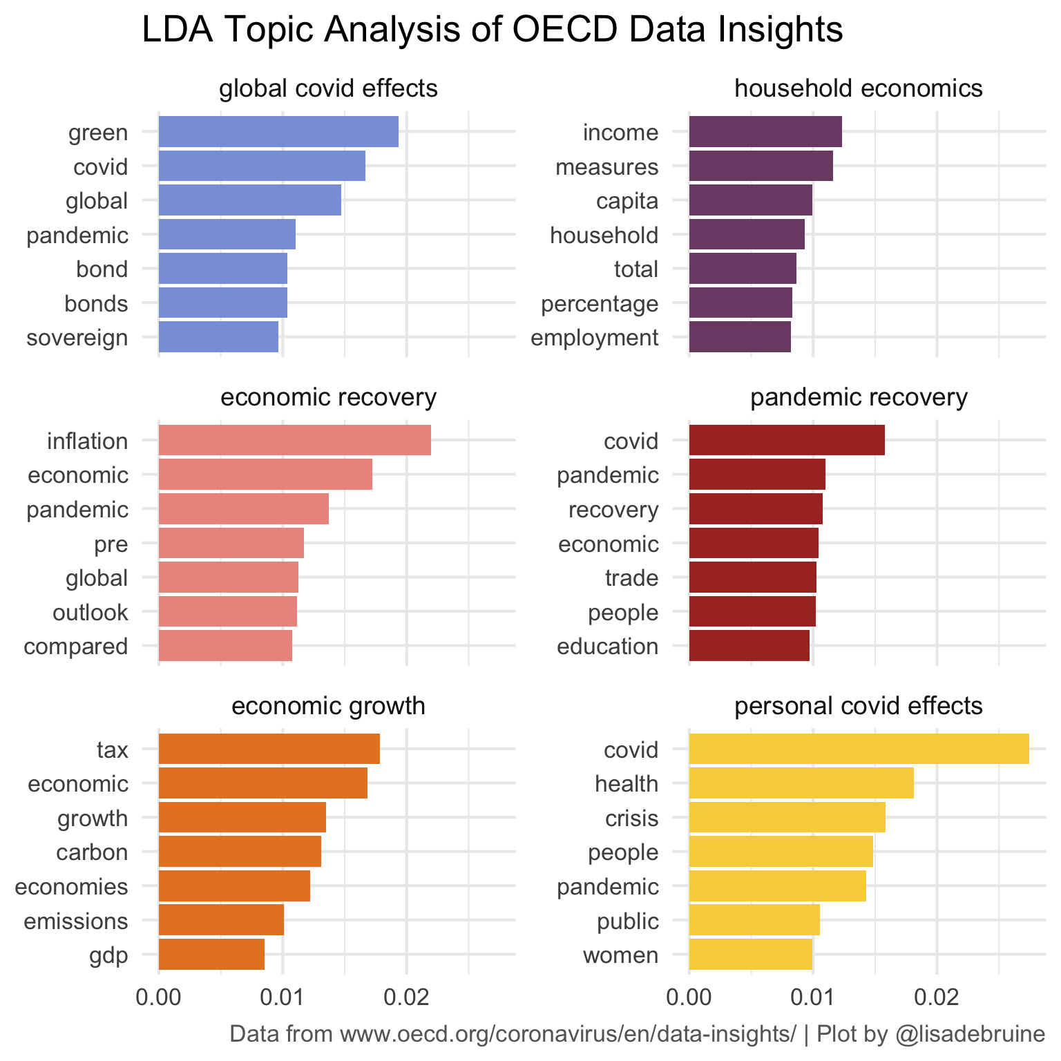
Get the top 7 terms for each topic.

Code

top_terms <- tidy(lda, matrix = "beta") %>%
  group_by(topic) %>%
  slice_max(beta, n = 7) %>% 
  ungroup() %>%
  arrange(topic, -beta)

top_terms %>%
  group_by(topic) %>%
  summarise(words = paste(term, collapse = ", "))

topic	words
1	green, covid, global, pandemic, bond, bonds, sovereign
2	income, measures, capita, household, total, percentage, employment
3	inflation, economic, pandemic, pre, global, outlook, compared
4	covid, pandemic, recovery, economic, trade, people, education
5	tax, economic, growth, carbon, economies, emissions, gdp
6	covid, health, crisis, people, pandemic, public, women

18.2.3 Document Topics

Now we need to figure out what these topics are. I don’t have a great sense from the top words, so we’ll can also make a table of gammas, which score each “document” (url in our case) on each of the 6 topics.

Code

gammas <- tidy(lda, matrix = "gamma") %>%
  mutate(title = gsub("https://www.oecd.org/coronavirus/en/data-insights/", 
                      "", document, fixed = TRUE))

Then determine the main topic for each document and plot the topic mix for each document, grouped by main topic.

Code

gammas %>%
  group_by(title) %>%
  mutate(main_topic = max(gamma) == gamma,
         main_topic = ifelse(main_topic, topic, 0),
         main_topic = sum(main_topic)) %>%
  ungroup() %>%
  ggplot(aes(x = title, y = gamma, fill = as.factor(topic))) +
  geom_col() +
  coord_flip() +
  scale_x_discrete(labels = rev)+
  MetBrewer::scale_fill_met_d("Archambault") +
  labs(x = NULL, fill = "Topic") +
  facet_wrap(~main_topic, scales = "free", ncol = 1) +
  theme(legend.position = "top")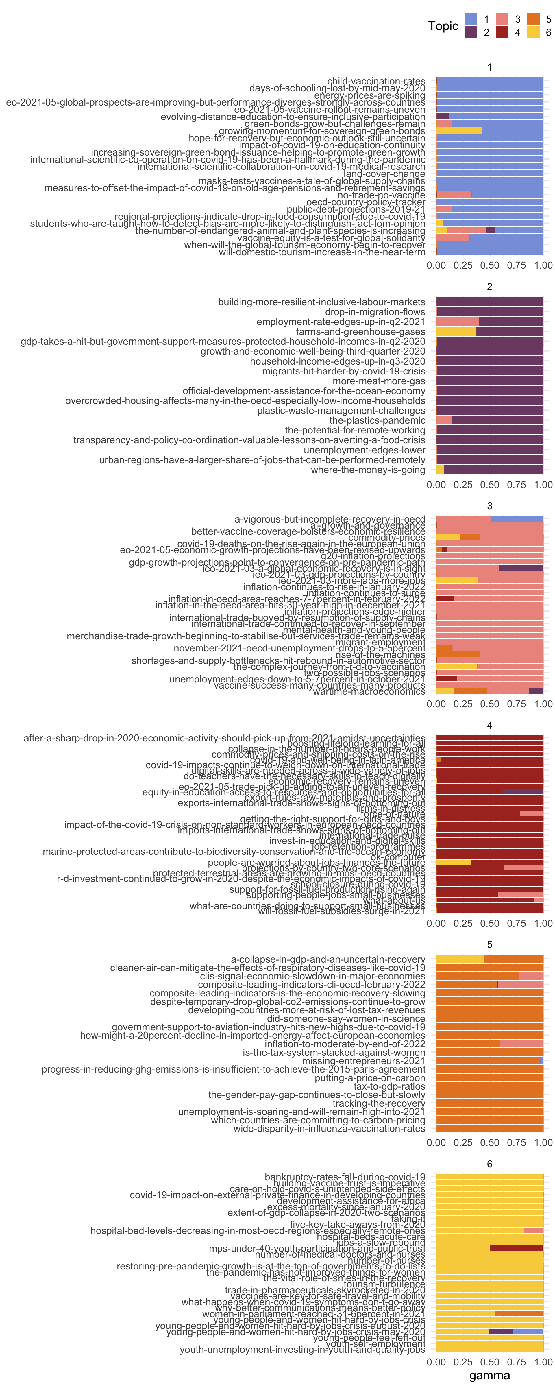

18.2.4 Add Topic Labels

After looking at the table above, there are my best guesses for topic labels. Update the facet labels with the as_labeller() function.

Code

topics <- c("global covid effects",
            "household economics",
            "economic recovery",
            "pandemic recovery",
            "economic growth",
            "personal covid effects")
names(topics) <- 1:6

top_terms %>%
  mutate(term = reorder_within(term, beta, topic)) %>%
  ggplot(aes(beta, term, fill = factor(topic))) +
  geom_col(show.legend = FALSE) +
  facet_wrap(~ topic, scales = "free_y", nrow = 3,
             labeller = as_labeller(topics)) +
  scale_x_continuous(breaks = seq(0, 1, .01)) +
  scale_y_reordered() +
  labs(x = NULL, y = NULL,
       title = "LDA Topic Analysis of OECD Data Insights",
       caption = "Data from www.oecd.org/coronavirus/en/data-insights/ | Plot by @lisadebruine") +
  MetBrewer::scale_fill_met_d("Archambault") +
  theme(plot.title = element_text(size = 20),
        plot.caption = element_text(color = "grey40"),
        strip.text = element_text(size = 14))

LDA Topic Analysis of OECD Data Insights