26  Interactive

I’m going to make a shiny app of a few of my previous charts in this challenge for interactive day. I’ll be using a lot of resources from my book,

Setup

#remotes::install_github("debruine/shinyintro")
library(tidyverse)     # for data wrangling and viz
library(sf)            # for maps
library(rnaturalearth) # for map coordinates
library(ggthemes)      # for map theme
library(lwgeom)        # for map projection
library(shinyintro)    # for shiny app template
library(tictoc)        # for timing things
library(tidytext)      # for text analysis
library(topicmodels)   # for topic modelling
library(MetBrewer)     # for beautiful colourblind-friendly colour schemes

26.1 Set up shiny app

You can do all this manually, but my shinyintro companion package to the book has a function to set up the skeleton of an app exactly how I like it.

Code

shinyintro::clone(app = "basic_template", dir = "app")

Here are the files it installs:

Code

list.files("app", full.names = TRUE, recursive = TRUE)

 [1] "app/app.R"                                           
 [2] "app/data/oecd_covid_insights.rds"                    
 [3] "app/data/share-of-individuals-using-the-internet.csv"
 [4] "app/data/world.rds"                                  
 [5] "app/DESCRIPTION"                                     
 [6] "app/README.md"                                       
 [7] "app/rsconnect/shinyapps.io/debruine/30DCC.dcf"       
 [8] "app/scripts/func.R"                                  
 [9] "app/www/basic_template.css"                          
[10] "app/www/custom.css"                                  
[11] "app/www/custom.js"                                   
[12] "app/www/img/30DCC.png"                               
[13] "app/www/img/psyteachr.png"                           
[14] "app/www/img/shinyintro.png"                          

26.2 App structure

Next, I’ll edit the README.md and DESCRIPTION files to describe my app and update the app.R file for my new app structure. The skeleton app code is for a tabbed interface using shinydashboard. I’ll set the skin to purple, change the demo_tab to an intro_tab and add a tab for day6, the first chart I’m going to make interactive.

Tabs Code

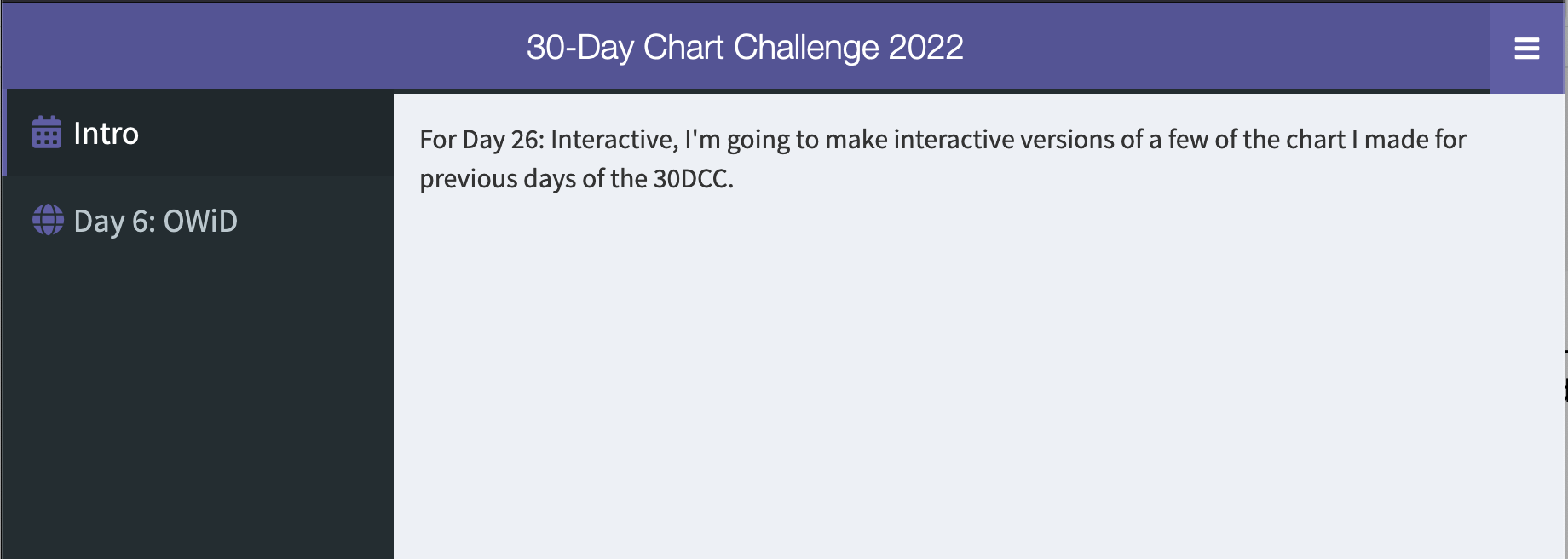
## tabs ----
intro_tab <- tabItem(
  tabName = "intro_tab",
  p("For Day 26: Interactive, I'm going to make interactive versions of a few of the charts I made for previous days of the 30DCC."),
  img(src = "img/30DCC.png", width = 500, height = 500)
)

day6 <- tabItem(
    tabName = "day6"
)

I like to define my tabs as objects so I can easily move them to a separate file and source them in when the amount of code gets overwhelming. I also have to add menuItems for these tabs to the dashboardPage() sidebar, find icons at fontawesome, and add the tab objects into tabItems() in the dashboardBody().

UI Code

## UI ----
ui <- dashboardPage(
    skin = "purple",
    dashboardHeader(title = "30-Day Chart Challenge 2022", 
        titleWidth = "calc(100% - 44px)" # puts sidebar toggle on right
    ),
    dashboardSidebar(
        # https://fontawesome.com/icons?d=gallery&m=free
        sidebarMenu(
            id = "tabs",
            menuItem("Intro", tabName = "intro_tab", icon = icon("calendar")),
            menuItem("Day 6: OWiD", tabName = "day6", icon = icon("globe"))
        )
    ),
    dashboardBody(
        shinyjs::useShinyjs(),
        tags$head(
            # links to files in www/
            tags$link(rel = "stylesheet", type = "text/css", href = "basic_template.css"), 
            tags$link(rel = "stylesheet", type = "text/css", href = "custom.css"), 
            tags$script(src = "custom.js")
        ),
        tabItems(
          intro_tab, day6
        )
    )
)

This is what the app looks like at this point when you run it:

26.3 Day 6

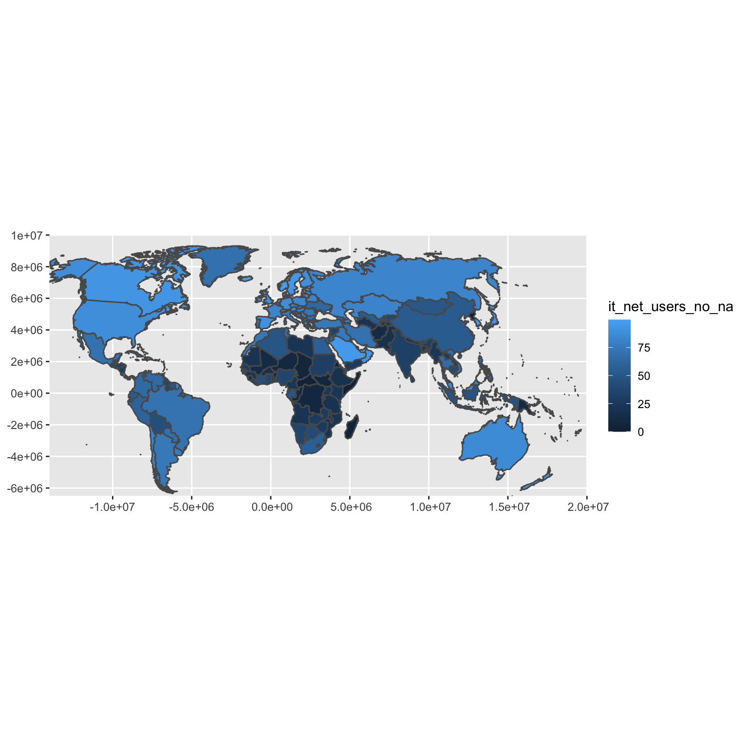
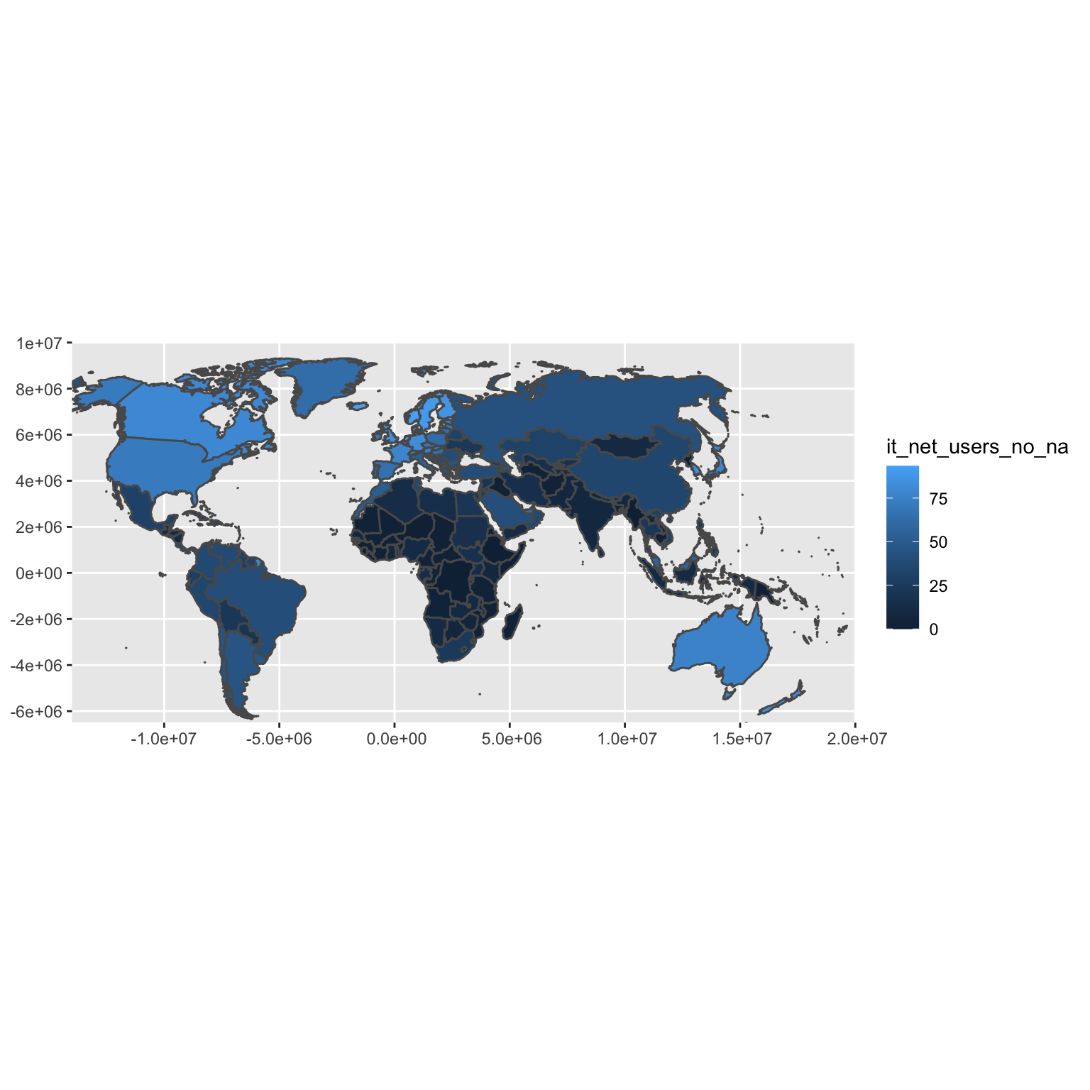
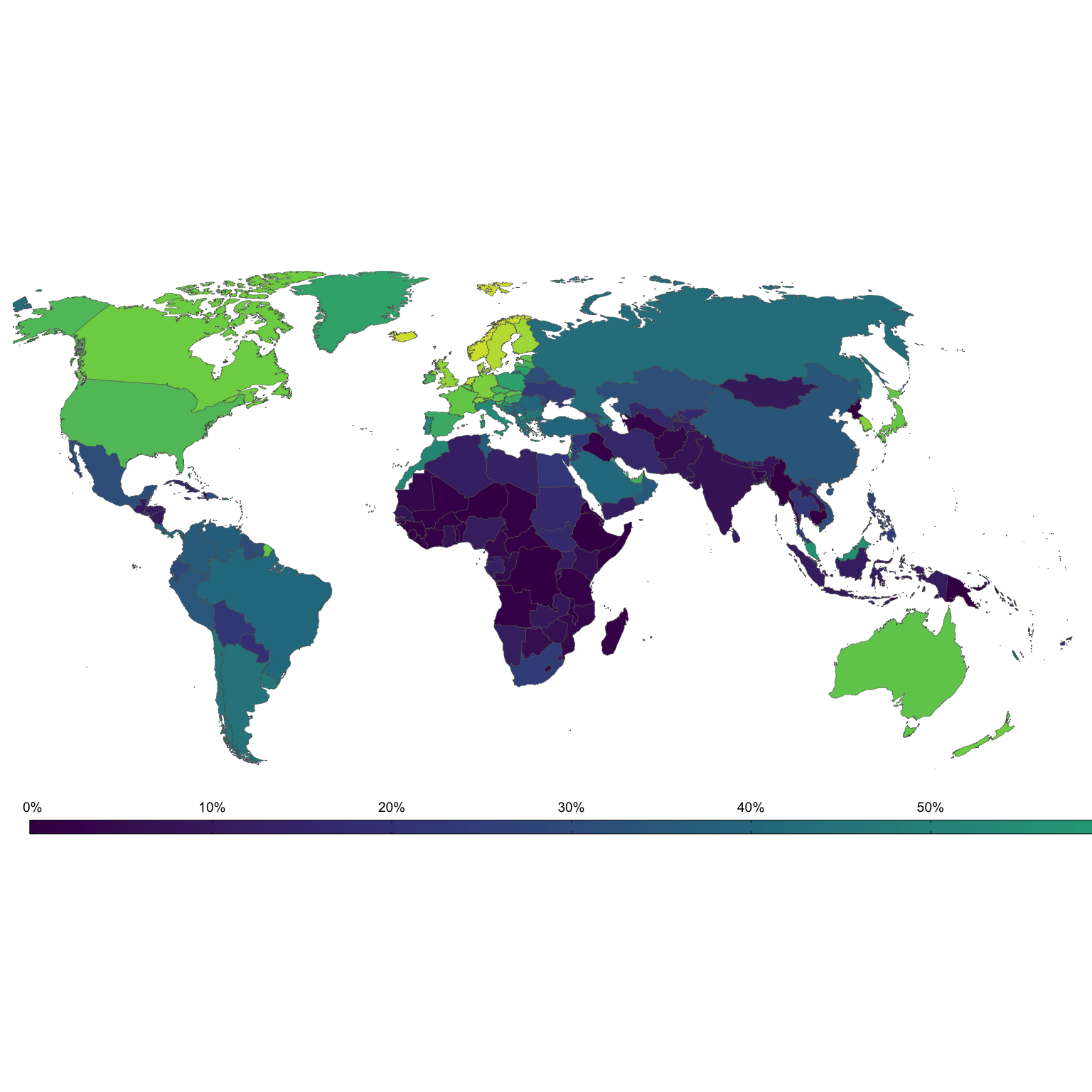
This was originally an animated map showing the share of the population using the internet in every country from 1990 to 2019. My plan is to make this interactive by adding a slider so you can pick the year.

26.3.1 Map functions

I like to keep as much code as possible out of the app.R file, so I’m going to add some functions to the scripts/func.R file to create the main plot. First, I need to create the dataset to be filtered.

day6_data()

day6_data <- function(crs = "+proj=wintri") {
  data_na <- read_csv("data/share-of-individuals-using-the-internet.csv",
                        col_names = c("country", "code", "year", "it_net_users"),
                        skip = 1, show_col_types = FALSE) %>%
    mutate(code = recode(code, SSD = "SDS", .default = code)) %>% 
    pivot_wider(names_from = year, 
                values_from = it_net_users) %>%
    pivot_longer(cols = -c(country, code),
                 names_to = "year",
                 values_to = "it_net_users", 
                 names_transform = list(year = as.integer))
  
  world <- ne_countries(returnclass = "sf", scale = "medium") %>%
    lwgeom::st_transform_proj(crs = crs)
  
  data_map_int_no_missing <- left_join(world, data_na, 
                            by = c("gu_a3" = "code")) %>%
    select(country, year, code = gu_a3, it_net_users, geometry) %>%
    filter(!is.na(year)) %>%
    mutate(it_net_users_no_na = it_net_users,
           missing = is.na(it_net_users)) %>%
    arrange(code, year) %>%
    group_by(country) %>%
    fill(it_net_users_no_na, .direction = "down") %>%
    ungroup()
  
  # fix south sudan
  sudan <- data_map_int_no_missing %>%
    filter(country == "Sudan",
           year <= 2012) %>%
    pull(it_net_users_no_na)

  ss_rows <- which(data_map_int_no_missing$country == "South Sudan" & 
                   data_map_int_no_missing$year <= 2012)
  
  nona <- data_map_int_no_missing$it_net_users_no_na
  nona[ss_rows] <- sudan
  
  data_map_int_final <- data_map_int_no_missing %>%
    mutate(it_net_users_no_na = nona)
  
  data_map_int_final
}

I also need to make a function to get the crop coordinates for the projection I’m using.

crop_coords()

crop_coords <- function(crs = "+proj=wintri") {
  # translate and crop coordinates
  trans_coords <- st_sfc(
    st_point(c(-1.4e7, -6.5e6)), # lower left lat and lon
    st_point(c(2e7, 1e7)),       # upper right lat and lon
    crs = crs) %>%
    st_transform(crs = crs) %>%
    st_coordinates()
  
  coord_sf(
    datum = NULL, 
    xlim = trans_coords[,'X'], 
    ylim = trans_coords[,'Y'], 
    expand = FALSE
  )
}

Test the functions in a simple plot.

Plot Test

day6_data() %>%
  filter(year == 2019) %>%
  ggplot() + 
  geom_sf(mapping = aes(fill = it_net_users_no_na)) +
  crop_coords()

Write a plotting function that takes the year as an argument.

Demo Plot Function

day6_plot <- function(filter_year = 2019) {
  day6_data() %>%
  filter(year == filter_year) %>%
  ggplot() + 
  geom_sf(mapping = aes(fill = it_net_users_no_na)) +
  crop_coords()
}

tictoc::tic()
day6_plot()

Demo Plot Function

tictoc::toc()

1.935 sec elapsed

This is pretty slow. What can we do to speed it up? Maybe make the day6 data first?

Time Data Loading

tictoc::tic("process data")
day6_data <- day6_data()
tictoc::toc()

process data: 0.476 sec elapsed

Time Plot Function

day6_plot <- function(data, filter_year = 2019) {
  data %>%
    filter(year == filter_year) %>%
    ggplot() + 
    geom_sf(mapping = aes(fill = it_net_users_no_na)) +
    crop_coords()
}

tictoc::tic("build demo plot")
day6_plot(day6_data, 2010)

Time Plot Function

tictoc::toc()

build demo plot: 1.315 sec elapsed

Nope, reading the data isn’t adding much to the plotting time, but half a send faster is still better. Maybe we’ll come back to this. Add the rest of the plot functions.

day6_plot()

day6_plot <- function(data, filter_year = 2019) {
  data %>%
    filter(year == filter_year) %>%
    ggplot() + 
    geom_sf(mapping = aes(fill = it_net_users_no_na/100),
            size = .1) +
    crop_coords() +
    scale_fill_viridis_c(
      name = NULL,
      limits = c(0, 1),
      breaks = seq(0, 1, .1),
      labels = function(x) scales::percent(x, accuracy = 1),
      guide = guide_colorbar(
        label.position = "top", 
        barheight = unit(.1, "in"),
        frame.colour = "black",
        ticks.colour = "black"
      )
    ) +
    ggthemes::theme_map() +
    theme(
      legend.background = element_blank(),
      legend.position = "bottom",
      legend.key.width = unit(.33, "snpc")
    )
}

tictoc::tic("build full plot")
day6_plot(day6_data, 2010)

day6_plot()

tictoc::toc()

build full plot: 0.497 sec elapsed

26.3.2 UI

I need to add an input and an output to the day 6 tab. Set sep = "" to remove the comma for the thousands separator, which makes no sense for years.

Day 6 UI

day6 <- tabItem(
    tabName = "day6",
    sliderInput("day6_year", 
                label = "Year", 
                min = 2009, 
                max = 2019, 
                value = 2019,
                step = 1, 
                sep = ""),
    plotOutput("day6_plot")
)

26.3.3 Server function

I also need to add the code to produce the output plot to the server function. I defined the data table day6_data outside the server function because this only needs to run once, when the app in initialised. There’s no reason to run it for every instantiation of the app or every time the plot is rendered.

Day 6 server function

day6_data <- day6_data()

# server ----
server <- function(input, output, session) {
    output$day6_plot <- renderPlot({
      day6_plot(day6_data, input$day6_year)
    })
}

Now I just need to add some title and caption text. It’s still a bit slow, but properly interactive. If this is all I needed it to do, I’d probably pre-render the chart for each of the 11 years at app startup and flip between the images rather than rerender the plot each time, but this is fine for today’s challenge.

26.4 Day 18

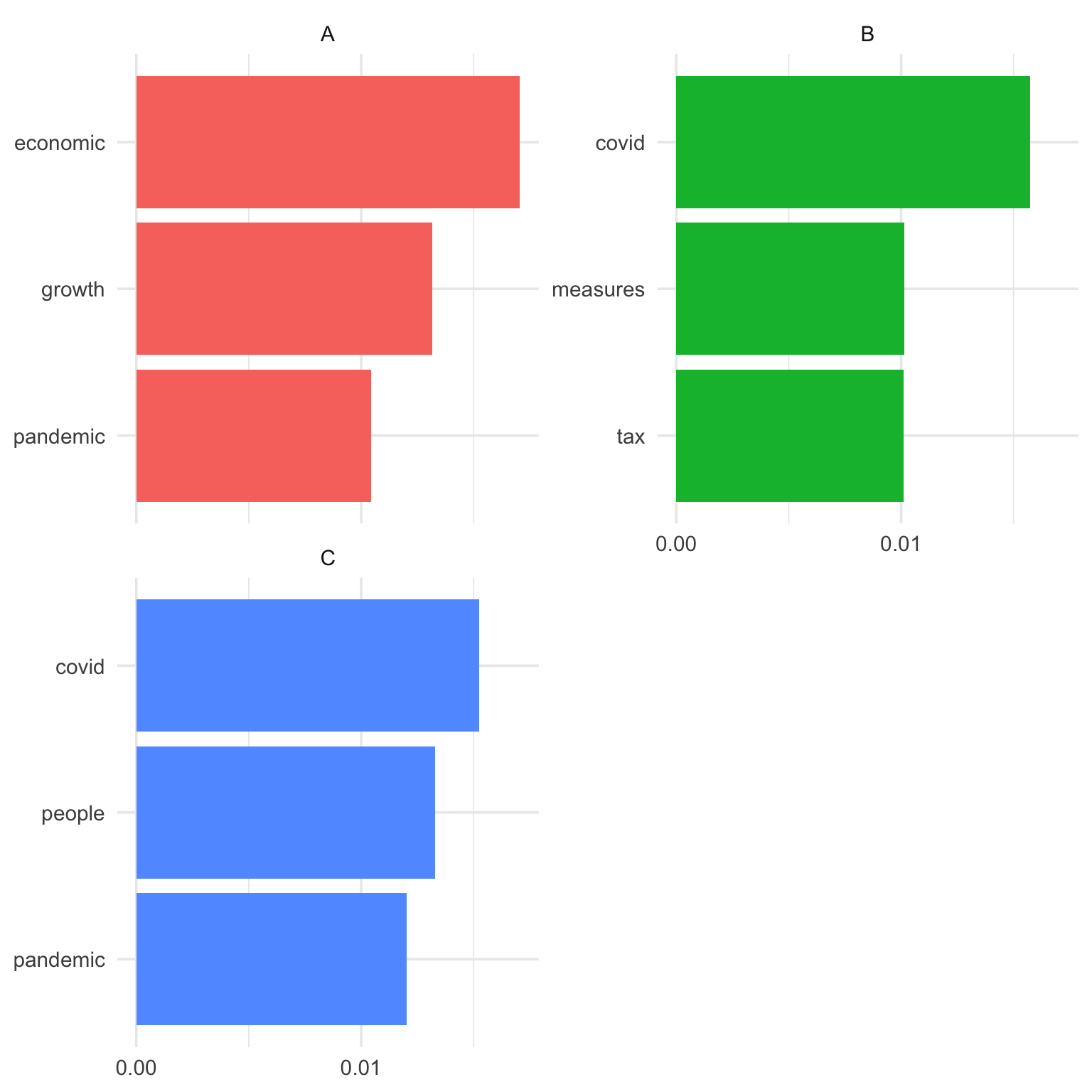
Day 18 was one where I had to look at a few different versions of the code and plot before deciding on some parameters, so let’s make those topic modelling parameters interactive.

26.4.1 Data Functions

We can greatly condense the code from Day 18.

Day 18 Data Functions

get_dtm <- function() {
  sw <- data.frame(word = c(stop_words$word, 0:2030, "oecd", "countries"))
  
  readRDS("data/oecd_covid_insights.rds") %>%
    filter(p != "Follow us (Social Media):") %>%
    unnest_tokens(word, p) %>%
    anti_join(sw, by = "word") %>%
    count(url, word, sort = TRUE) %>%
    cast_dtm(document = url, term = word, value = n)
}

get_lda <- function(dtm, k = 6) {
  dtm %>%
    LDA(k = k, control = list(seed = 8675309))
}

get_top_terms <- function(lda, n_terms = 7) {
  tidy(lda, matrix = "beta") %>%
  group_by(topic) %>%
  slice_max(beta, n = n_terms) %>% 
  ungroup() %>%
  arrange(topic, -beta)
}

Test the functions.

Code

lda3 <- get_lda(get_dtm(), k = 3)

tt3 <- get_top_terms(lda3, 3)

tt3

topic	term	beta
1	economic	0.017
1	growth	0.013
1	pandemic	0.010
2	covid	0.016
2	measures	0.010
2	tax	0.010
3	covid	0.015
3	people	0.013
3	pandemic	0.012

26.4.2 Plot Function

Day 18 Plot Function

day18_plot <- function(top_terms, topics = list()) {
  names(topics) <- seq_along(topics)
  
  top_terms %>%
    mutate(term = reorder_within(term, beta, topic)) %>%
    ggplot(aes(beta, term, fill = factor(topic))) +
    geom_col(show.legend = FALSE) +
    facet_wrap(~ topic, scales = "free_y", nrow = 2,
               labeller = as_labeller(topics)) +
    scale_x_continuous(breaks = seq(0, 1, .01)) +
    scale_y_reordered() +
    labs(x = NULL, y = NULL) +
    scale_fill_hue() +
    theme_minimal(base_size = 14)
}

Code

day18_plot(tt3, c("A", "B", "C"))

26.4.3 Setup

Now add the function to scripts/func.R and make sure to add the appropriate packages to the top of the app.R file. Add dtm <- dtm() to the top of the app.R script (after sourcing in func.R) because this only needs to be called once. Make sure to move oecd_covid_insights.rds to the app data folder.

26.4.4 UI

Same as above, make a new tab for day 18, with inputs and an output plot.

Day 18 UI

day18 <- tabItem(
  tabName = "day18",
  h2("LDA Topic Analysis of OECD Data Insights"),
  numericInput("day18_k", 
               label = "Number of Topics",
               min = 2, max = 16, value = 6, step = 1),
  numericInput("day18_topterms", 
               label = "Number of Terms per Topic",
               min = 1, max = 20, value = 7, step = 1),
  textAreaInput("day18_topics", 
                label = "Topic Labels (one per line)",
                rows = 6),
  plotOutput("day18_plot"),
  HTML("<caption>Data from <a href='https://www.oecd.org/coronavirus/en/data-insights/'>OECD</a> | Plot by <a href='https://twitter.com/lisadebruine'>@lisadebruine</a></caption>")
)

26.4.5 Server function

Set up the render function for the plot.

Day 18 server function

output$day18_plot <- renderPlot({
  lda <- get_lda(dtm, k = input$day18_k)
  tt <- get_top_terms(lda, input$day18_topterms)
  topics <- strsplit(input$day18_topics, split = "\n")[[1]] %>% 
    trimws() %>%
    rep(length.out = input$day18_k)
  day18_plot(tt, topics)
})

26.4.6 Test and Update

After a few tests, I realised that I needed to remove the constraint of nrow = 2 in the facet_wrap() and also restructure how I was splitting the string in the topic labels to deal with blank lines or too few/many labels.

I also decided it was too annoying waiting for the whole plot to update every time I wanted to change the topic labels, so restructured the server code to only rerun code when absolutely necessary, and to add an update button for the topic labels, so they only update when you’re done editing the labels.

The reactive() functions only run when the inputs or reactive functions they contain update, while the observeEvent() function only runs when the input value for the first argument changes.

Day 18 server function updates

    # topic_labels ----
    topic_labels <- reactiveVal(c("global covid effects",
                                     "household economics",
                                     "economic recovery",
                                     "pandemic recovery",
                                     "economic growth",
                                     "personal covid effects"))
    
    # day18_update_topics ----
    observeEvent(input$day18_update_topics, {
      paste0(input$day18_topics, " ") %>%
        strsplit(split = "\n") %>%
        `[[`(1) %>% 
        trimws() %>%
        rep(length.out = input$day18_k) %>%
        topic_labels()
    })
    
    # lda ----
    lda <- reactive({ get_lda(dtm, k = input$day18_k) })
    
    # tt ----
    tt <- reactive({ get_top_terms(lda(), input$day18_topterms) })
    
    # plot18 ----
    plot18 <- reactive({ day18_plot(tt(), topic_labels()) })
    
    # day18_plot ---- 
    output$day18_plot <- renderPlot({ plot18() })

I also added a download button to the UI and a download handler to the server function.

Day 18 Download

    # day18_dl ----
    output$day18_dl <- downloadHandler(
      filename = function() {
        "OECD_topic_model.png"
      },
      content = function(file) {
        ggsave(file, plot18())
      }
    )

26.5 Deploy App

I currently don’t have access to our work shiny server because of some server changes, so I deployed the app at debruine.shinyapps.io/30DCC.

It didn’t work the first time, and I realised that I only use one function each from rnaturalearth and lwgeom, so I saved world as an RDS object and loaded it from the saved file instead of using those packages.

Code

# world <- rnaturalearth::ne_countries(returnclass = "sf", scale = "medium") %>%
#   lwgeom::st_transform_proj(crs = crs)
# saveRDS(world, "data/world.rds")
world <- readRDS("data/world.rds")

That stopped the total app failure, but the day18 chart still wouldn’t build, so I added debug messages to the day18 functions so I could see what was and wasn’t running.

The debug_msg() function is a custom function that prints the debug message in the console during development, and in the javascript console when deployed (in case you don’t have access to the logs). The code below prints “day18_topterms” whenever the tt() reactive function runs, and if there is an error in the code, tryCatch() catches it and prints the error message with debug_msg(). This way, I discovered that I was getting an error “there is no package called ‘reshape2’”, so I added that to the library() calls at the start of the script.

Code

# tt ----
tt <- reactive({ debug_msg("day18_topterms")
  tryCatch( 
    get_top_terms(lda(), input$day18_topterms),
    error = function(e) debug_msg(e$message) 
  )
})

Now it works!