4 Flora
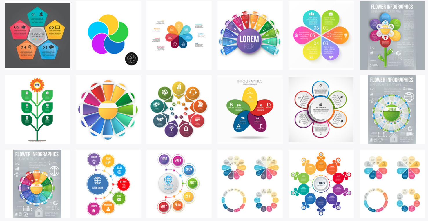
I’m going a little off-piste today. I was inspired by all of these stock infographics, but I wondered if I could make something similar with code. You probably can do this with ggplot and annotations, but I wanted to try something different.
4.1 SVG
I have some experience making SVGs (scalable vector graphics), but I always have to look things up. W3Schools is my favourite source for quick tutorials on web stuff. I used it a ton to make this chart.
While I was developing this code, I needed to have a quick look at the images a lot, and couldn’t figure out an efficient way to view SVGs, so I wrote a function that converts the svg text to a PNG tempfile and displays it in my Rmd, but only when I’m running the code interactively.
SVG viewer function
viewsvg <- function(svg, width = 5, height = 5, dpi = 150) {
  if (interactive() &&
      !isTRUE(getOption("knitr.in.progress"))) {
    imgpath <- tempfile(fileext = ".png")
    rsvg::rsvg_png(svg = charToRaw(svg),
                   file = imgpath,
                   width = width*dpi, height = height*dpi)
    knitr::include_graphics(imgpath)
  } else {
    cat(svg)
  }
}
It outputs the SVG as html when knitting. All of the images below are created with a code chunk that looks like this:
4.2 Flower Petals
First, I need a function to figure out the coordinates of regular polygons. Finally, high school trigonometry comes in handy!
Polygon coordinate function
$x
[1]  1.0  0.5 -0.5 -1.0 -0.5  0.5

$y
[1]  0.00  0.87  0.87  0.00 -0.87 -0.87
Now, make n circles with radius r that are petal_dist away from the center of the flower.
Code
n <- 6
r <- 200
petal_dist <- 300
cx <- 500
cy <- 500

coords <- poly_coords(n, petal_dist, cx, cy)
petals <- glue('    <circle cx="{coords$x}" cy="{coords$y}" r="{r}" fill="{rainbow(n)}" />') %>%
  paste(collapse = "\n")

svg <- paste("<svg viewBox = '0 0 {2*cx} {2*cy}'>",
        petals,
      "</svg>",
      sep = "\n") %>%
  glue()
4.3 Rotate
Rotate them so the red is at 12:00.
4.4 Fix the Overlap
When they overlap, the last petal is on top of the first, so we need to replot the left half of that. It took me forever to figure out how to plot the left half of a circle with <path> :(
Code
coords <- poly_coords(n, petal_dist, cx, cy, rot)
petals <- glue('    <circle cx="{coords$x}" cy="{coords$y}" r="{r}" fill="{rainbow(n)}" />') %>%
  paste(collapse = "\n")

x1 <- coords$x[[1]]
y1 <- coords$y[[1]]
petal_fix <- glue('    <g transform="rotate({rot*180/pi}, {x1}, {y1})">
       <path d="M {x1-r} {y1}
       A {r} {r} 0 0 1 {x1+r} {y1}
       L {x1-r} {y1}
       Z"
       fill="{rainbow(n)[[1]]}" /></g>')

svg <- paste("<svg viewBox = '0 0 {2*cx} {2*cy}'>",
        petals, petal_fix,
      "</svg>",
      sep = "\n") %>%
  glue()
Now I want to add a center hexagon that just touches each petal.
4.5 7 Petals
Code
n          <- 7
rot        <- 8.5*pi/7
petal_dist <- 400
r          <- 200
cx         <- 1.1 * (petal_dist + r)
cy         <- cx

center <- poly_coords(n, petal_dist-r, cx, cy, rot) %>%
  glue("{cc$x},{cc$y}", cc = .) %>%
  paste(collapse = " ") %>%
  glue('<polygon points="{pts}" fill="grey" />', pts = .)

coords <- poly_coords(n, petal_dist, cx, cy, rot)
petals <- glue('    <circle cx="{coords$x}" cy="{coords$y}" r="{r}" fill="{rainbow(n)}" />') %>%
  paste(collapse = "\n")

x1 <- coords$x[[1]]
y1 <- coords$y[[1]]
petal_fix <- glue('    <g transform="rotate({rot*180/pi}, {x1}, {y1})">
       <path d="M {x1-r} {y1}
       A {r} {r} 0 0 1 {x1+r} {y1}
       L {x1-r} {y1}
       Z"
       fill="{rainbow(n)[[1]]}" /></g>')


text <- glue('    <text x="{coords$x}" y="{coords$y+40}">{LETTERS[1:n]}</text>"') %>%
  paste(collapse = "\n")

svg_style <- '<style type="text/css">
svg {
  font-family: sans-serif;
  font-size: 80px;
  text-anchor: middle;
  fill: white;
}
</style>'

svg <- paste("<svg viewBox = '0 0 {{2*cx}} {{2*cy}}'>",
             svg_style,
             center,
             '<text x="{{cx}}" y="{{cy-20}}">All of the</text>',
             '<text x="{{cx}}" y="{{cy+90}}">Things</text>',
             petals, petal_fix, text, "</svg>",
             sep = "\n") %>%
glue(.open = "{{", .close = "}}")4.6 Make a Function
Now I just need to wrap this all in a function so I can change the things I need. I also added transparency to the petals, which necessitated making the two halves of the first petal separately, otherwise the overlap fix increases the opacity of half the petal if there’s any transparency.
Code
poly_coords <- function(n = 6, r = 1, cx = 0, cy = 0, rot = 0, digits = 2) {
  x = map_dbl(0:(n-1), ~{ cx + r * cos(2 * pi * .x / n + rot) })
  y = map_dbl(0:(n-1), ~{ cy + r * sin(2 * pi * .x / n + rot) })

  list(
    x = round(x, digits),
    y = round(y, digits)
  )
}

flower <- function(n = 6, petal_dist = 500, r = 250, rot = -pi/2,
                   petal_text = LETTERS[1:n],
                   center_text = c("All of the", "Things"),
                   petal_text_size = r/2,
                   center_text_size = petal_dist/6,
                   center_text_offsets = c(-0.2, +0.9) * center_text_size,
                   petal_colors = rainbow(n),
                   petal_alpha = 1.0,
                   center_color = "#808080",
                   petal_text_color = "white",
                   center_text_color = petal_text_color) {

  # calculate centre
  cx <- 1.1 * (petal_dist + r)
  cy <- cx

  # make centre polygon
  center <- poly_coords(n, petal_dist-r, cx, cy, rot) %>%
    glue("{cc$x},{cc$y}", cc = .) %>%
    paste(collapse = " ") %>%
    glue('<polygon points="{pts}" fill="{center_color}" />', pts = .)

  # make center texts
  center_texts <- glue('    <text x="{cx}" y="{cy+center_text_offsets}" fill="{center_text_color}" font-size="{center_text_size}px">{center_text}</text>') %>%
    paste(collapse = "\n")

  # make petals
  coords <- poly_coords(n, petal_dist, cx, cy, rot)
  petals <- glue('    <circle cx="{coords$x}" cy="{coords$y}" r="{r}" fill="{petal_colors}" fill-opacity="{petal_alpha}" />') %>%
    paste(collapse = "\n")

  x1 <- coords$x[[1]]
  y1 <- coords$y[[1]]
  petal_fix1 <- glue('    <g transform="rotate({(rot+pi)*180/pi}, {x1}, {y1})">
         <path d="M {x1-r} {y1}
         A {r} {r} 0 0 1 {x1+r} {y1}
         L {x1-r} {y1}
         Z"
         fill="{petal_colors[[1]]}" fill-opacity="{petal_alpha}" /></g>')

  petal_fix2 <- glue('    <g transform="rotate({rot*180/pi}, {x1}, {y1})">
         <path d="M {x1-r} {y1}
         A {r} {r} 0 0 1 {x1+r} {y1}
         L {x1-r} {y1}
         Z"
         fill="{petal_colors[[1]]}" fill-opacity="{petal_alpha}" /></g>')

  # make petal text
  petals_text <- glue('    <text x="{coords$x}" y="{coords$y+petal_text_size/2}">{petal_text}</text>', .literal = TRUE) %>%
    paste(collapse = "\n")

  # general styles
  svg_style <- '<style type="text/css">
  svg {
    font-family: sans-serif;
    font-size: {{petal_text_size}}px;
    text-anchor: middle;
    fill: {{petal_text_color}};
  }
</style>'

  svg <- paste("<svg viewBox = '0 0 {{2*cx}} {{2*cy}}'>",
               svg_style,
               center, center_texts,
               petal_fix1, petals, petal_fix2, petals_text,
               "</svg>",
               sep = "\n") %>%
    glue(.open = "{{", .close = "}}")

  svg
}
Test the defaults.
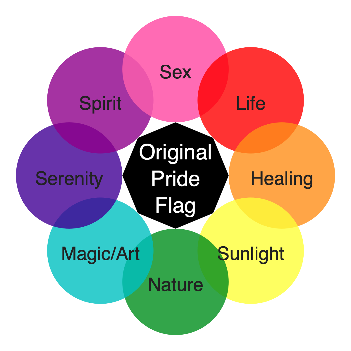
4.7 Original Pride Flag
Test the customisability by making a chart with the meaning of the 8 colours of the original pride flag.
Code
svg <- flower(n = 8, petal_dist = 400, r = 200,
              petal_colors = c("#FF66B1", "#FF0000", "#FF8F1A", "#FEFF3A",
                               "#008F1D", "#00C0C0", "#420095", "#8F008B"),
              petal_alpha = 0.8,
              petal_text = c("Sex", "Life", "Healing", "Sunlight",
                             "Nature", "Magic/Art", "Serenity", "Spirit"),
              center_text = c("Original", "Pride", "Flag"),
              center_text_size = 80,
              center_text_offsets = c(-60, 40, 140),
              petal_text_color = "#222222",
              petal_text_size = 70,
              center_color = "black",
              center_text_color = "white"
)4.8 Save as SVG or PNG
You can display your SVG directly in a website by setting results='asis' in the code chunk header. It will display it full size unless you use another method to constrain the image size. I set a css style of svg { width: 100%; }.
You can write it to an svg file, or use svgr to convert to an image.