17  Connections

I’ve been meaning to learn more about visualising text, and where better to start than Julia Silge and David Robinson’s Text Mining with R!

Setup

library(tidyverse) # always useful
library(tidytext)  # for text analysis
library(ggraph)    # for plotting ngrams
library(showtext)  # for custom fonts
library(ggtext)    # for adding the twitter logo

font_add("arista", "fonts/arista_light.ttf")
font_add("fa-brands", "fonts/fa-brands-400.ttf")
showtext_auto()

17.1 Data

I’ll be using my own tweets from 2021. I have a tutorial in the Applied Data Skills book on how to get these data and process them.

Load data

tweet_files <- list.files(
  path = "data/tweets", 
  pattern = "^tweet_activity_metrics",
  full.names = TRUE
)

ct <- cols("Tweet id" = col_character())

tweets <- map_df(tweet_files, read_csv, col_types = ct) %>%
  select(text = `Tweet text`)

17.2 Bigrams

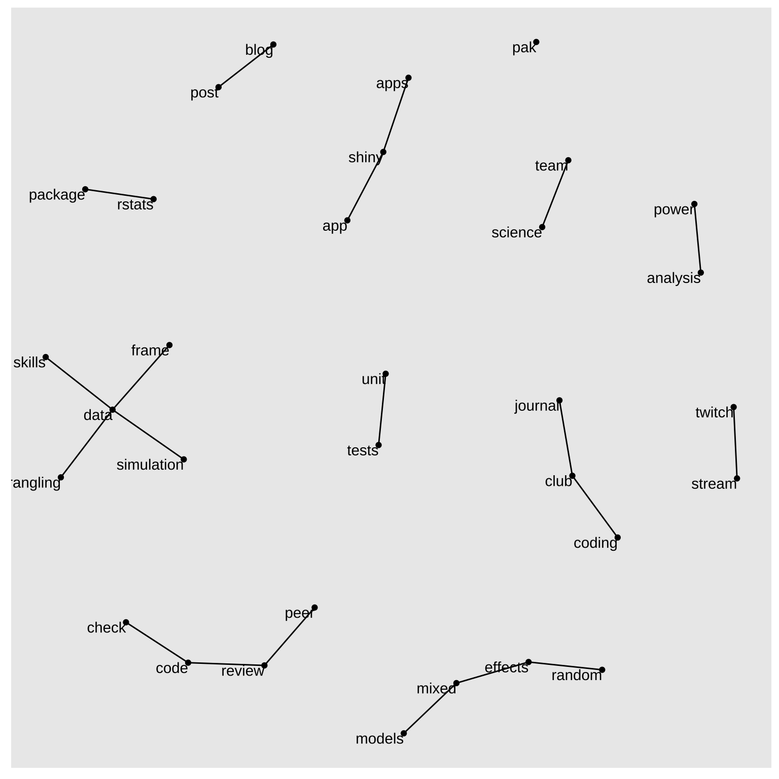
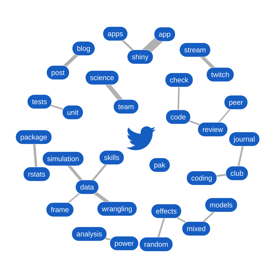
Here I used the code from the ngrams chapter to get a table of all the word pairs in my tweets. I added one line to get rid of all the twitter usernames (i.e., any word that starts with @).

Code

bigrams <- tweets %>%
  mutate(no_usernames = gsub("@[A-Za-z_0-9]+", "", text)) %>%
  unnest_tokens(bigram, no_usernames, token = "ngrams", n = 2)

bigram_counts <- bigrams %>% 
  count(bigram, sort = TRUE)

head(bigram_counts, 10)

bigram	n
https t.co	1306
in the	282
of the	282
if you	149
to be	149
to the	149
you can	142
but i	141
this is	139
in a	129

The most common ones are stop words, so separate the words into word1 and word2 and get rid of any rows without words (e.g., 1-word tweets). I added a few custom entries to the stop_words$words list: “https”, “t.co”, “gt”, “lt”, and the numbers 0 to 100.

Code

bigrams_separated <- bigrams %>%
  separate(bigram, c("word1", "word2"), sep = " ") %>%
  filter(!is.na(word1), !is.na(word2))

my_stop_words <- c(stop_words$word, "https", "t.co", "gt", "lt", 0:100, "00")

bigrams_filtered <- bigrams_separated %>%
  filter(!word1 %in% my_stop_words) %>%
  filter(!word2 %in% my_stop_words)

bigram_counts <- bigrams_filtered %>% 
  count(word1, word2, sort = TRUE)

head(bigram_counts)

word1	word2	n
shiny	app	45
team	science	26
blog	post	21
data	wrangling	21
twitch	stream	20
data	simulation	18

17.3 Plot ngrams

First, I’ll follow the chapter example to create a basic plot.

Code

bigram_graph <- bigram_counts %>%
  filter(n > 10)

Code

set.seed(8675309)

ggraph(bigram_graph, layout = "fr") +
  geom_edge_link() +
  geom_node_point() +
  geom_node_text(aes(label = name), vjust = 1, hjust = 1)

The word “pak” looks all by itself because, for no reason I can recall, I tweeted “pak pak” 11 times last year.

17.4 Tidy the plot

As always, now it’s time to make the plot prettier.

I tried a bunch of layouts (see ?layout_tbl_graph_igraph) and the spring-based algorithm by Kamada and Kawai (“kk”) looked best.

Add a bit of padding to the margins and set coord_cartesian(clip = "off") to avoid clipping labels that are too close to the edge.

I added the twitter logo to the middle using ggtext and Albert Rapp’s tutorial.

Code

ggraph(bigram_graph, layout = "kk") +
  geom_edge_link(aes(width = n), color = "grey", show.legend = FALSE) +
  geom_node_label(aes(label = name), vjust = 0.5, hjust = 0.5,
                  fill = "dodgerblue3", color = "white", 
                  label.padding = unit(.5, "lines"),
                  label.r = unit(.75, "lines")) +
  annotate("richtext", label = "<span style='font-family:fa-brands'>&#xf099;</span>",
           x = 0.3, y = -.2, col = 'dodgerblue3', label.colour = NA,
           family='fa-brands', size=16) +
  coord_cartesian(clip = "off") +
  theme_void() +
  theme(plot.margin = unit(rep(.5, 4), "inches"))

Bigram graph of my 2021 tweets.