24  Financial Times

Setup

library(tidyverse) # for data wrangling
library(readxl)    # for reading data from WHO
library(patchwork) # for combining plots
library(ggtext)    # for styled text in plots
library(showtext)  # for fonts

font_add_google("Roboto", regular.wt = 300, bold.wt = 500)
font_add_google("Roboto", family = "RobotoB", regular.wt = 400, bold.wt = 700)
showtext_auto()

24.1 Examples

I browsed the Financial Times Data Visualisation webpage to find a plot I want to re-create. I don’t have a subscription, so I could only see the thumbnails, but it looks like this is a section for snarky commentary on plots.

I did find that you can hack the image URLs to increase the width and see bigger versions.

Code

# download.file("https://www.ft.com/__origami/service/image/v2/images/raw/https%3A%2F%2Fd1e00ek4ebabms.cloudfront.net%2Fproduction%2Fdfac7f09-aaca-4e94-b4eb-b96180e69a8a.png?source=next&fit=scale-down&dpr=2&width=1200", "images/ft_whirlwind.png")
knitr::include_graphics("images/ft_whirlwind.png")

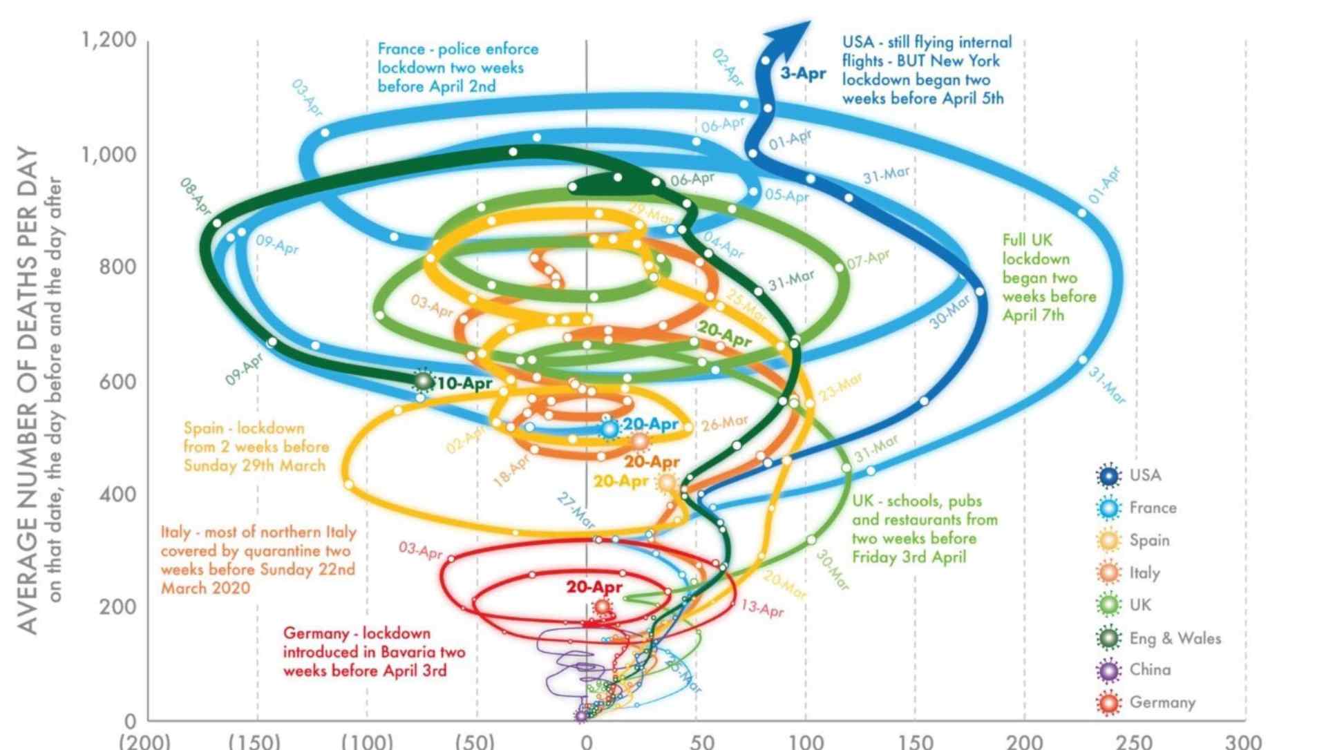
I don’t think I’ll be trying to re-create this plot

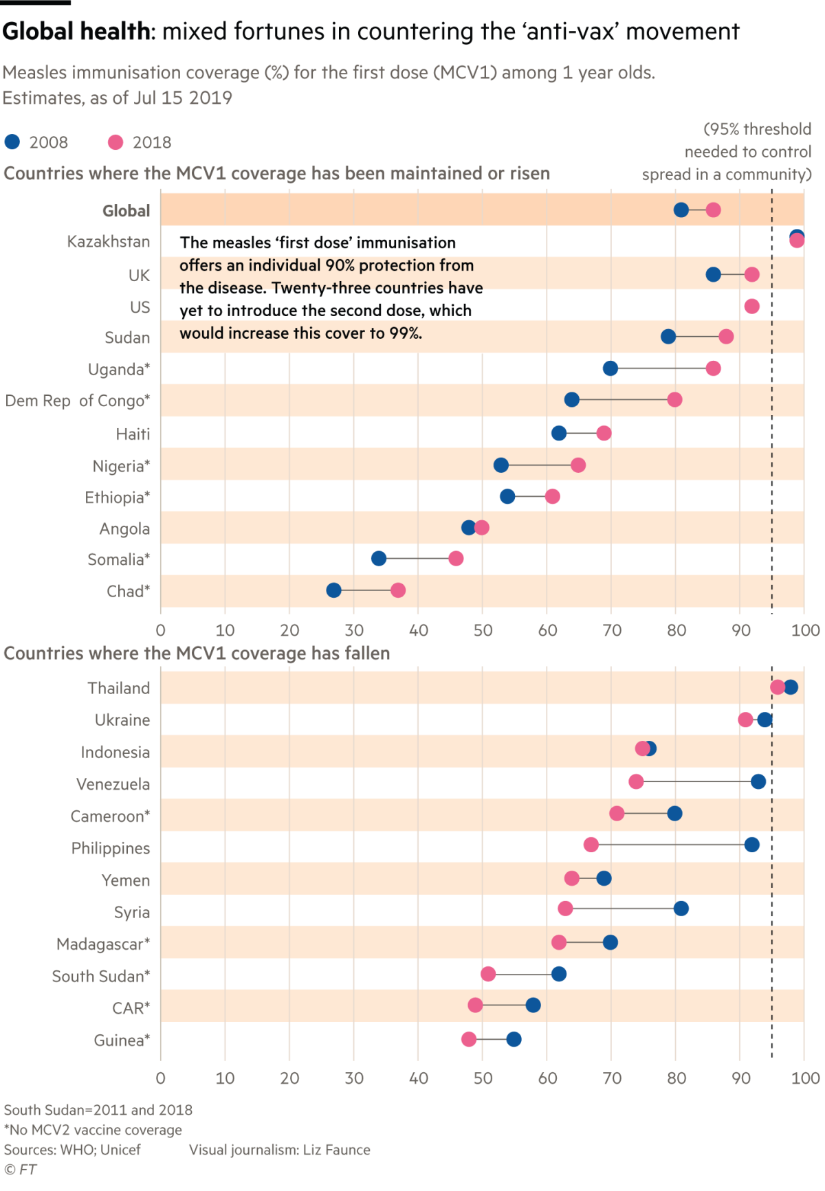
The Visual and data journalism section looks more fruitful, if I had a subscription. Then I searched twitter (congrats on getting a 2-letter handle, @FT!) and found a link to an article on Ten charts that tell the story of 2019 that I could access. It’s interesting to read some pre-pandemic news; the first two charts are on Brexit and anti-vax movements.

I always like these lollipop charts and haven’t had much practice making them, so I’m going to recreate this plot.

24.2 Data

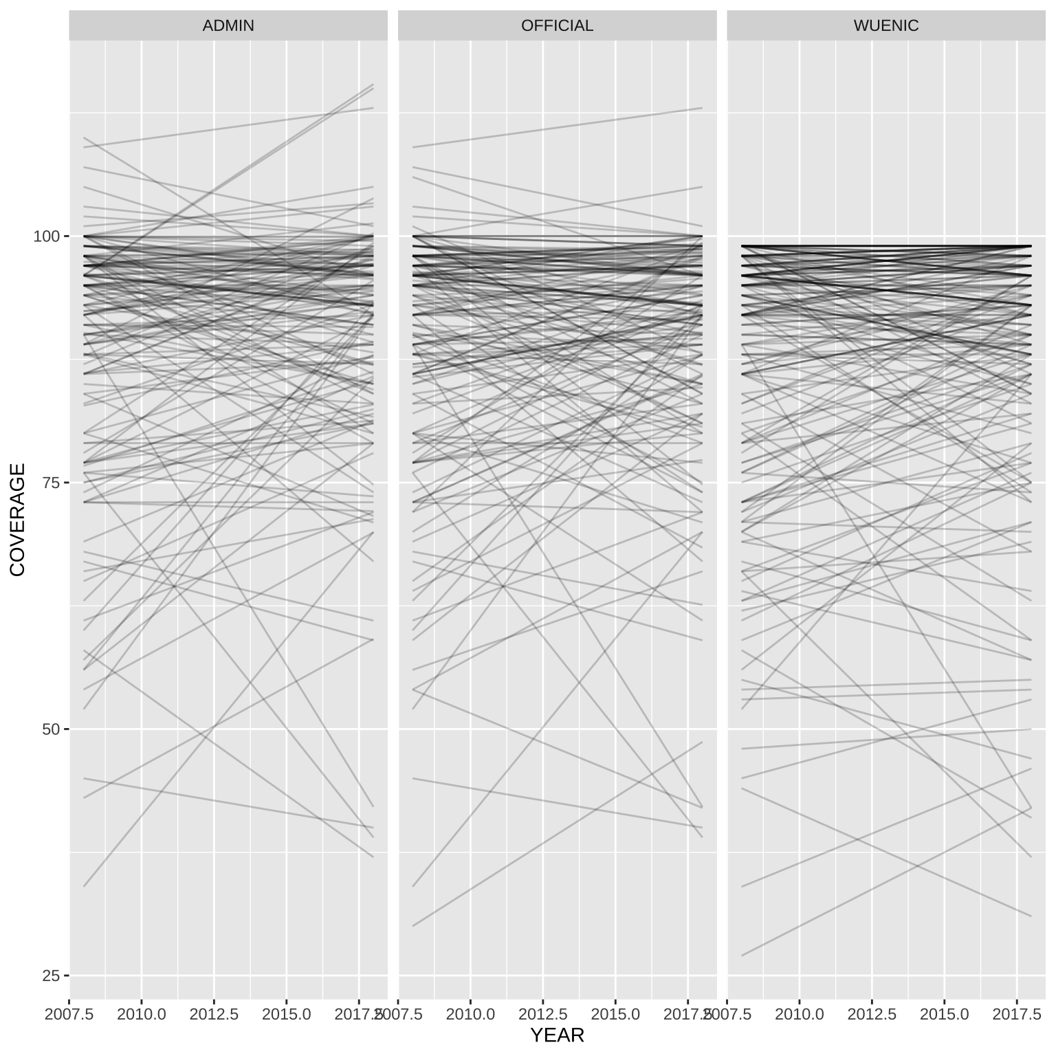
First, I needed to find the data. The original chart said the data came from WHO and Unicef; I downloaded the WHO Data on MCV1.

Code

measles <- read_xlsx("data/Measles vaccination coverage.xlsx")

mcv1 <- measles %>%
  select(CODE, NAME, YEAR, COVERAGE_CATEGORY, COVERAGE) %>%
  filter(YEAR %in% c(2008, 2018))

head(mcv1)

CODE	NAME	YEAR	COVERAGE_CATEGORY	COVERAGE
AFG	Afghanistan	2018	ADMIN	82.45
AFG	Afghanistan	2008	ADMIN	75.00
AFG	Afghanistan	2018	OFFICIAL	82.00
AFG	Afghanistan	2008	OFFICIAL	59.00
AFG	Afghanistan	2018	WUENIC	71.00
AFG	Afghanistan	2008	WUENIC	59.00

24.2.1 Pick a coverage category

I’m not sure what the different coverage categories are, but a quick plot shows that the WUENIC values are at least all under 100%.

Code

ggplot(mcv1, aes(x = YEAR, y = COVERAGE, group = NAME)) +
  geom_line(alpha = 0.2) +
  facet_wrap(~COVERAGE_CATEGORY)

24.2.2 South Sudan

I need to use the 2011 value for South Sudan instead of 2008, since South Sudan didn’t exist until 2011.

Code

ssd_2011 <- measles %>%
  filter(CODE == "SSD", 
         COVERAGE_CATEGORY == "WUENIC", 
         YEAR == 2011) %>%
  pull(COVERAGE)

mcv1 <- mcv1 %>%
  add_row(CODE = "SSD",
          NAME = "South Sudan",
          COVERAGE_CATEGORY = "WUENIC", 
          YEAR = 2008,
          COVERAGE = ssd_2011)

24.2.3 Choose focus countries

I tried to get the list of countries shown on the original chart programatically, but they’re not just the biggest increases and decreases, so I had to extract them manually. I wrote a quick function to search for the code for any name or part of a name.

Code

ccode <- function(txt) { 
  filter(mcv1, grepl(txt, NAME)) %>% 
    select(NAME, CODE) %>% 
    distinct() 
}

ccode("Congo")

NAME	CODE
Congo	COG
Democratic Republic of the Congo	COD

Some of the countries on the chart use different names or abbreviations, so I made a named vector with the country codes and names for the chart.

Code

countries <- c(
  Global = "Global", 
  KAZ = "Kazakhstan", 
  GBR = "UK", 
  USA = "USA", 
  SDN = "Sudan", 
  UGA = "Uganda", 
  COD = "Dem Rep of Congo", 
  HTI = "Haiti", 
  NGA = "Nigeria", 
  ETH = "Ethiopia", 
  AGO = "Angola", 
  SOM = "Solmalia", 
  TCD = "Chad", 
  THA = "Thailand", 
  UKR = "Ukraine", 
  IDN = "Indonesia", 
  VEN = "Venezuela", 
  CMR = "Cameroon", 
  PHL = "Philippines", 
  YEM = "Yemen", 
  SYR = "Syria", 
  MDG = "Madagascar", 
  SSD = "South Sudan", 
  CAF = "Ctl African Rep", 
  GIN = "Guinea"
)

I used that vector to filter the mcv1 table, make a new column called country and make it a factor so the countries will display in the right order. I also filtered the table to just the “WUENIC” coverage and made the table wide so there was a column for each year.

Code

mcv1_status <- mcv1  %>%
  filter(CODE %in% names(countries)) %>%
  mutate(country = recode(CODE, !!!countries),
         country = factor(country, countries)
  ) %>%
  arrange(country) %>%
  filter(COVERAGE_CATEGORY == "WUENIC") %>%
  select(-COVERAGE_CATEGORY, -NAME) %>%
  pivot_wider(names_from = YEAR,
              names_prefix = "Y",
              values_from = COVERAGE) %>%
  drop_na() %>%
  mutate(change = ifelse((Y2018 - Y2008) < 0, "decrease", "increase"))

24.3 Plot

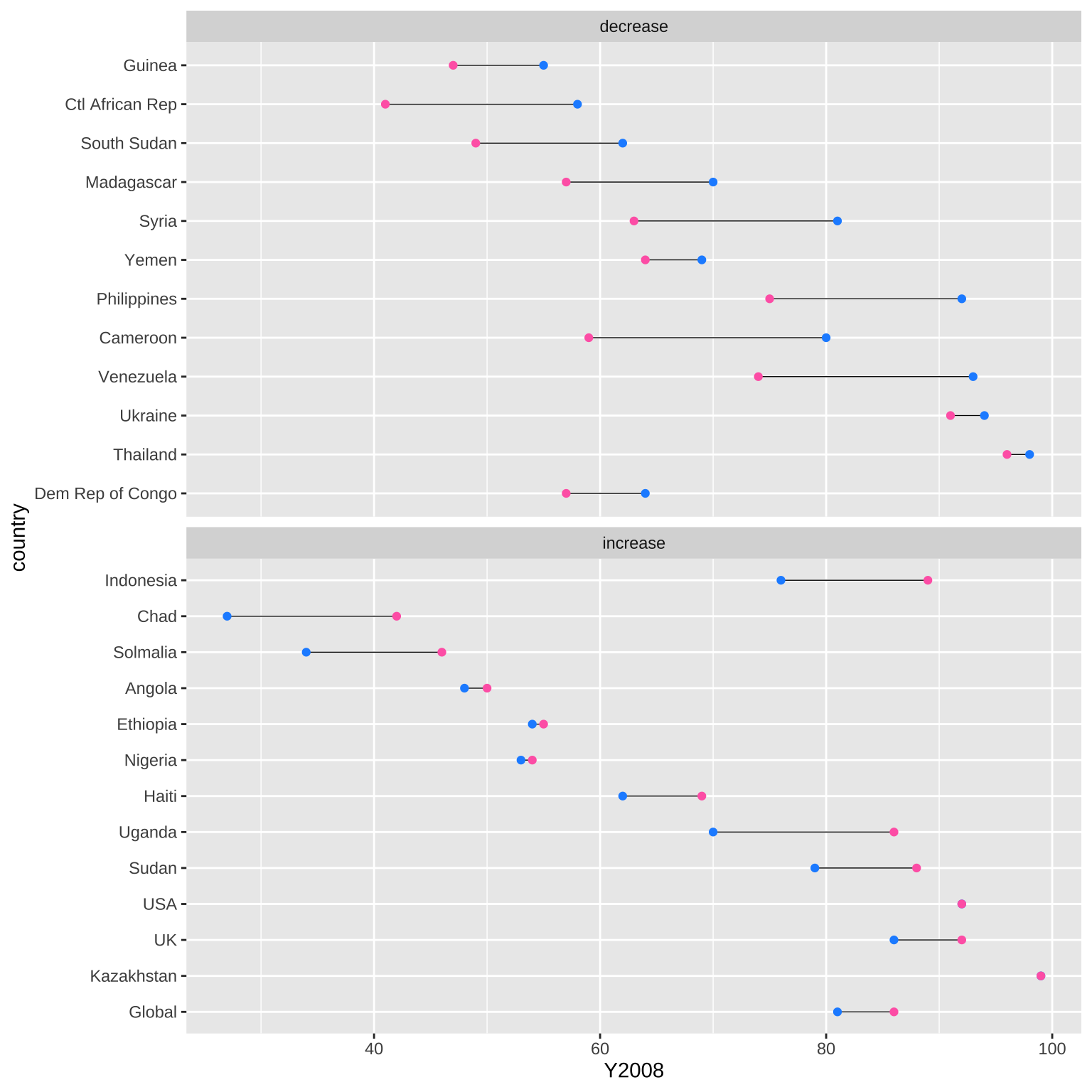
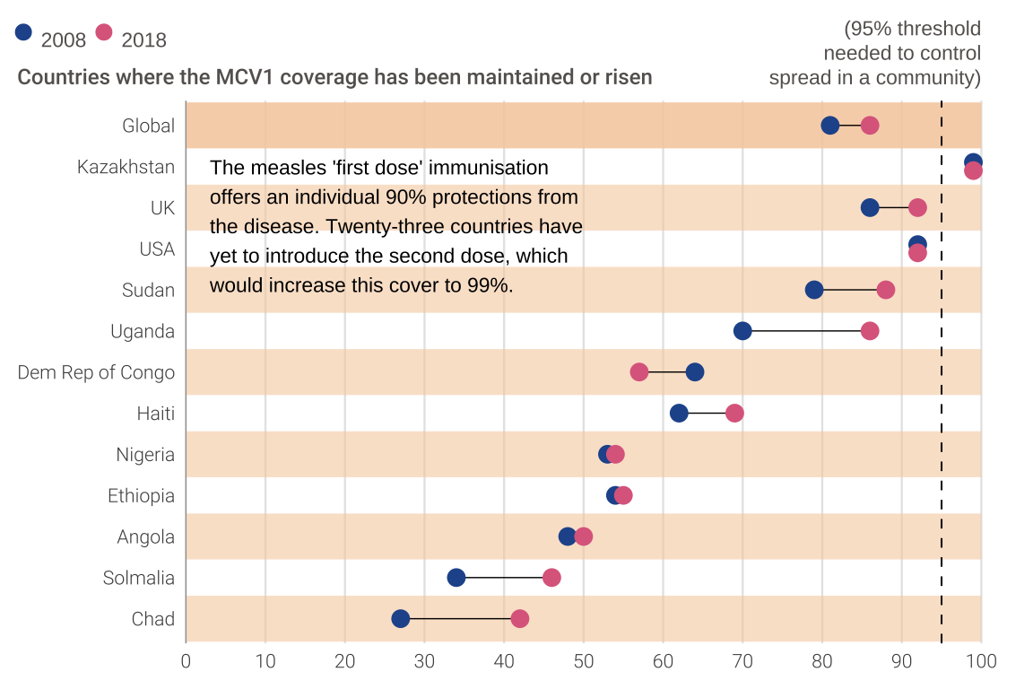
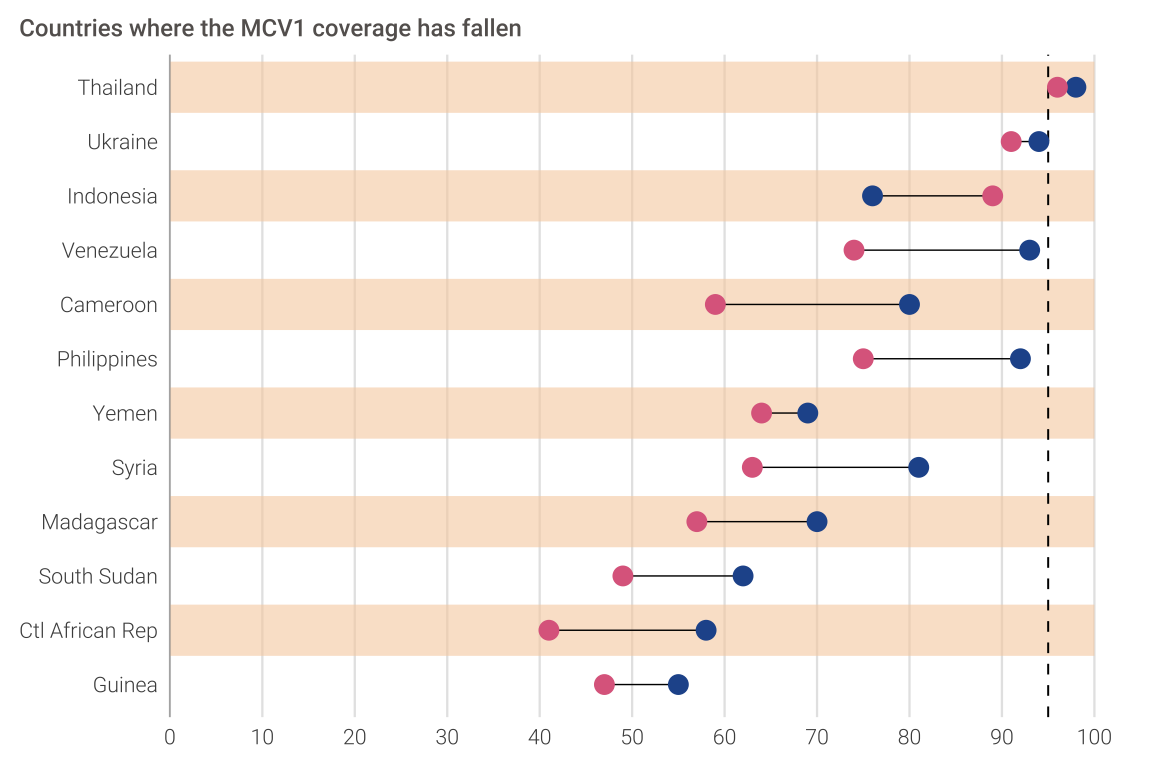
Time for the first plot! The data aren’t exactly the same as on the original chart. While the original chart showed an increase in vaccination in the Democratic Republic of the Congo, the data I’m using show a decrease. Similarly, Indonesia has a change in the opposite direction as the original chart. I’ll plot the data I have, but in the order of the original plot, so I’ll need to make two separate plots and combine them with patchwork.

Code

ggplot(mcv1_status, aes(y = country)) +
  geom_segment(aes(x = Y2008, xend = Y2018, yend = country), 
               color = "black", size = 0.25) +
  geom_point(aes(x = Y2008), color = "dodgerblue") +
  geom_point(aes(x = Y2018), color = "hotpink") +
  facet_wrap(~change, nrow = 2, scales = "free_y")

24.3.1 Theme

First, I need to set up a few things for the plot theme. I extracted the colour for the dots for 2008 and 2018, plus the background and stripe colours, and the grey text colour, and set those to variables I can use later.

Code

dot_08 <- "#24559A"
dot_18 <- "#DD6A8D"
bg_light <- "#FFFFFF" # "#FFF1E5" # FT website bg colour
bg_tan <- "#F6D0AE"
text_color <- "#65615E"

24.3.2 Overlap and stripes

In the original chart, Kazakhstan doesn’t have much change at all, so the dots are nudged up and down vertically so they don’t completely overlap. The USA also doesn’t have discernible change and isn’t nudged in the original plot, but I’ll nudge it here. I’ll make a new variable called y, which is the numeric value for the country factor, but reversed, and y08 and y18 which are the y-axis values for each year. They’re all the same as y, except for Kazakhstan and the USA.

I’ll also add a new column called stripe to set the alpha for the stripe for each country, following the pattern from the original chart, with Global being a dark stripe, and alternating semi-transparent and no stripe after that.

Code

figdat <- mcv1_status %>%
  mutate(
    y = rev(as.numeric(country)),
    y08 = y + ifelse(CODE %in% c("USA", "KAZ"), .1, 0),
    y18 = y - ifelse(CODE %in% c("USA", "KAZ"), .1, 0),
    stripe = c(0.9, 
               rep(c(0, 0.6), length.out = 12), 
               rep(c(0.6, 0), length.out = 12)
               )
  )

24.3.3 Risen plot

This plot took a lot of trial and error with the annotations. The trick is to set coord_cartesian(clip = "off") so you can plot outside the axis limits, and add some plot margin with the theme().

Code

# define top panel
risen <- slice(figdat, 1:13) %>%
  ggplot(aes(y = y)) +
  geom_hline(aes(yintercept = y, alpha = I(stripe)),
             color = bg_tan, size = 9) +
  geom_vline(xintercept = 95, linetype = 2, size = 0.35) +
  geom_segment(aes(x = Y2008, xend = Y2018, yend = y), 
               color = "black", size = 0.25) +
  geom_point(aes(x = Y2008, y = y08), 
             color = dot_08, size = 3) +
  geom_point(aes(x = Y2018, y = y18), 
             color = dot_18, size = 3) +
  annotate("text", size = 3,
           label = "The measles 'first dose' immunisation\noffers an individual 90% protections from\nthe disease. Twenty-three countries have\nyet to introduce the second dose, which\nwould increase this cover to 99%.", 
           x = 3, y = 24.15, hjust = 0, vjust = 1) +
  annotate("text", size = 3, 
           label = "(95% threshold\nneeded to control\nspread in a community)", 
           x = 100, y = 26, hjust = 1, vjust = 0, 
           lineheight = 1, color = text_color) +
  annotate("richtext", size = 3,
           label = "<span style='color: #24559A; font-size: 22px;'>●</span> 2008 <span style='color: #DD6A8D; font-size: 22px;'>●</span> 2018",
           x = -23, y = 26.5, hjust = 0, vjust = 0, 
           color = text_color,
           label.colour = "transparent") +
  scale_x_continuous(breaks = (0:10)*10, 
                     expand = expansion(0)) +
  scale_y_continuous(breaks = 1:25, 
                     labels = rev(figdat$country),
                     expand = expansion(add = .6)) +
  coord_cartesian(xlim = c(0, 100), ylim = c(13, 25), clip = "off") +
  labs(x = NULL, y = NULL,
       title="Countries where the MCV1 coverage has been maintained or risen")

# define theme
ft_theme <- theme_minimal(base_family = "Roboto", base_size = 10) +
  theme(
    text = element_text(color = text_color),
    plot.background = element_rect(fill = bg_light, color = "transparent"),
    axis.line.y.left = element_line(color = "grey60", size = 0.2),
    axis.line.y.right = element_line(color = "grey60", size = 0.2),
    panel.grid.major.y = element_blank(),
    panel.grid.minor.x = element_blank(),
    panel.grid.minor.y = element_blank(),
    panel.grid.major.x = element_line(size = 0.4, color = "grey90"),
    plot.title.position = "plot",
    plot.title = element_text(size = 9, face = "bold")
  )

# display top panel with theme
top_panel <- risen + ft_theme + 
  theme(plot.margin = unit(c(.4, .3, .1, .1), "inches"))

top_panel

24.3.4 Fallen plot

The lower plot is a bit simpler, with fewer annotations.

Code

# define bottom panel
fallen <- slice(figdat, 14:25) %>%
  ggplot(aes(y = y)) +
  geom_hline(aes(yintercept = y, alpha = I(stripe)),
             color = bg_tan, size = 9) +
  geom_vline(xintercept = 95, linetype = 2, size = 0.35) +
  geom_segment(aes(x = Y2008, xend = Y2018, yend = y), 
               color = "black", size = 0.25) +
  geom_point(aes(x = Y2008, y = y08), 
             color = dot_08, size = 3) +
  geom_point(aes(x = Y2018, y = y18), 
             color = dot_18, size = 3) +
  scale_x_continuous(breaks = (0:10)*10, 
                     expand = expansion(0)) +
  scale_y_continuous(breaks = 1:25, 
                     labels = rev(figdat$country),
                     expand = expansion(add = .6)) +
  coord_cartesian(xlim = c(0, 100), ylim = c(1, 12), clip = "off") +
  labs(x = NULL, y = NULL,
       title="Countries where the MCV1 coverage has fallen")

# display bottom panel with theme
bottom_panel <- fallen + ft_theme + 
  theme(plot.margin = unit(c(.1, .3, .1, .1), "inches"))

bottom_panel

24.3.5 Combine Plots

Code

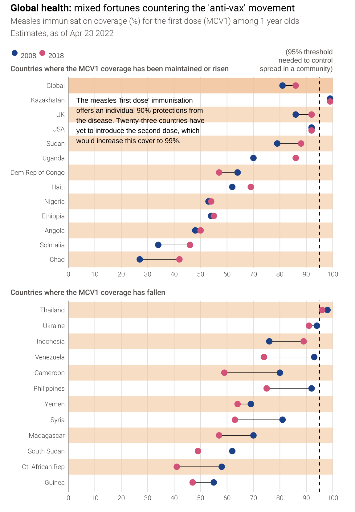
top_panel + bottom_panel +
  plot_annotation(
    title = "**Global health:** mixed fortunes countering the 'anti-vax' movement",
    subtitle = "Measles immunisation coverage (%) for the first dose (MCV1) among 1 year olds  \nEstimates, as of Apr 23 2022", 
    theme = theme(
      plot.background = element_rect(fill = bg_light, color = "transparent"),
      plot.title = element_markdown(size = 12, family = "RobotoB", 
                                    face = "plain", color = "black"),
      plot.subtitle = element_markdown(size = 10, family = "Roboto", 
                                       lineheight = 1.5,
                                       face = "plain", color = text_color)
    )
  ) +
  plot_layout(nrow = 2)