29  Storytelling

Storytelling makes me think of words, so this is another good opportunity to practice my text mining with Julia Silge and David Robinson’s Text Mining with R.

Setup

library(tidyverse) # for data wrangling
library(lubridate) # for handling dates
library(tidytext)  # for text analysis
library(textdata)  # for sentiment analysis

theme_set(theme_minimal(base_size = 16))

29.1 Data

I’m on a roll with this PsyArXiv data from Day 27, and it has a lot of text for the titles and descriptions (abstracts), so I’ll extract that.

Code

preprint_data <- readRDS("data/preprint_data.RDS")

info <- map_df(preprint_data, function(p) {
  list(id = p$id,
       pub_dt = p$attributes$date_published,
       title = p$attributes$title,
       desc = p$attributes$description
       )
}) %>%
  mutate(pub_dt = as_datetime(pub_dt))

29.2 Sentiment Analysis

I’ll use the sentiment analysis data from (mohammad13?), but convert it to wide format.

Code

wide_nrc <- get_sentiments("nrc") %>%
  mutate(x = TRUE) %>%
  pivot_wider(names_from = sentiment, 
              values_from = x,
              values_fill = FALSE)

head(wide_nrc)

word	trust	fear	negative	sadness	anger	surprise	positive	disgust	joy	anticipation
abacus	TRUE	FALSE	FALSE	FALSE	FALSE	FALSE	FALSE	FALSE	FALSE	FALSE
abandon	FALSE	TRUE	TRUE	TRUE	FALSE	FALSE	FALSE	FALSE	FALSE	FALSE
abandoned	FALSE	TRUE	TRUE	TRUE	TRUE	FALSE	FALSE	FALSE	FALSE	FALSE
abandonment	FALSE	TRUE	TRUE	TRUE	TRUE	TRUE	FALSE	FALSE	FALSE	FALSE
abba	FALSE	FALSE	FALSE	FALSE	FALSE	FALSE	TRUE	FALSE	FALSE	FALSE
abbot	TRUE	FALSE	FALSE	FALSE	FALSE	FALSE	FALSE	FALSE	FALSE	FALSE

I’ll work out the code I need on a small sample of the papers first, and them comment out slice_sample() after it looks like I expect. This takes a few second to run.

Code

sentiment <- info %>%
  #slice_sample(n = 1000) %>%
  unnest_tokens(word, desc) %>%
  inner_join(wide_nrc, by = "word") %>%
  group_by(id, title, pub_dt) %>%
  summarise(across(trust:anticipation, mean),
            .groups = "drop") %>%
  pivot_longer(cols = trust:anticipation,
               names_to = "sentiment",
               values_to = "value")

29.3 Plot

First let’s try a simple plot looking at how sentiments have changed over time.

Code

ggplot(sentiment, aes(x = pub_dt, y = value, color = sentiment)) +
  geom_smooth()

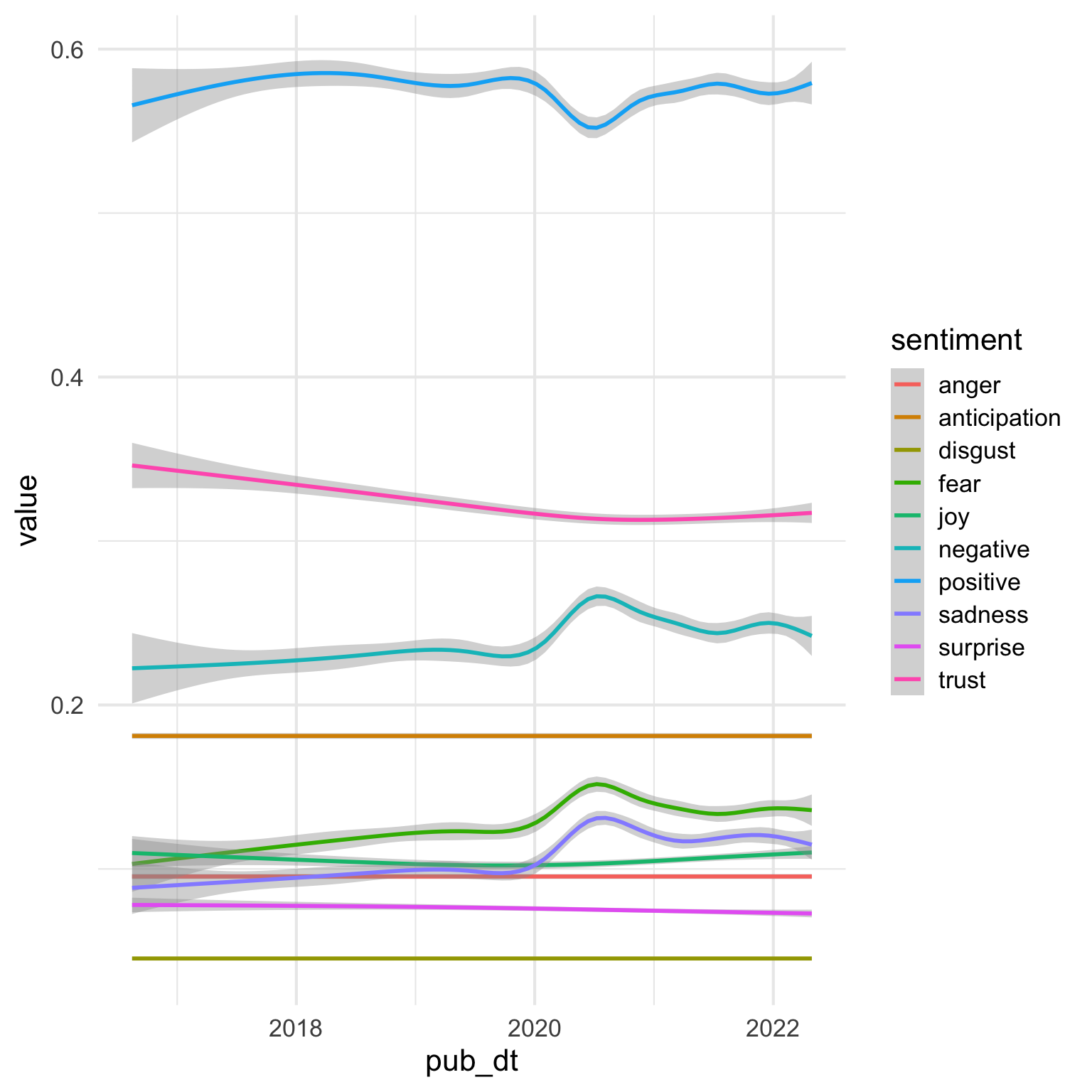
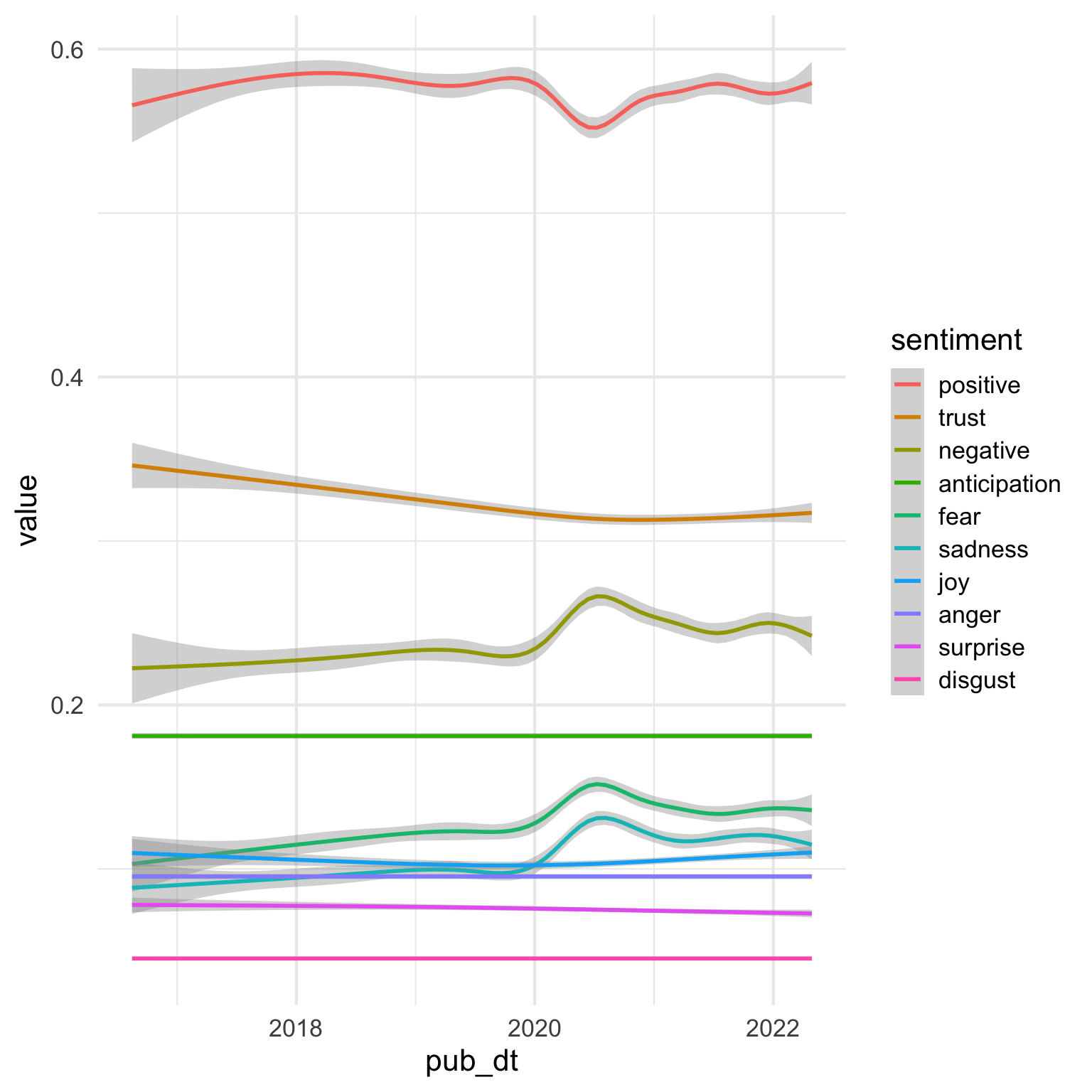
29.3.1 Fix sentiment order

The sentiments default to alphabetic order, but the plot would be easier to read if they were in order by prevalence. I’ll filter out the preprints from the most recent year and month, calculate the mean value for each sentiment, and arrange them in descending order. Then I can set the sentiment column as a factor with levels in this order.

Code

s_order <- sentiment %>%
  filter(year(pub_dt) == max(year(pub_dt))) %>% 
  filter(month(pub_dt) == max(month(pub_dt))) %>%
  group_by(sentiment) %>%
  summarise(v = mean(value), .groups = "drop") %>%
  arrange(desc(v))

sentiment$sentiment <- factor(sentiment$sentiment, 
                              levels = s_order$sentiment)

This gets them in the right order, but I still think we can do better.

Code

ggplot(sentiment, aes(x = pub_dt, y = value, color = sentiment)) +
  geom_smooth()

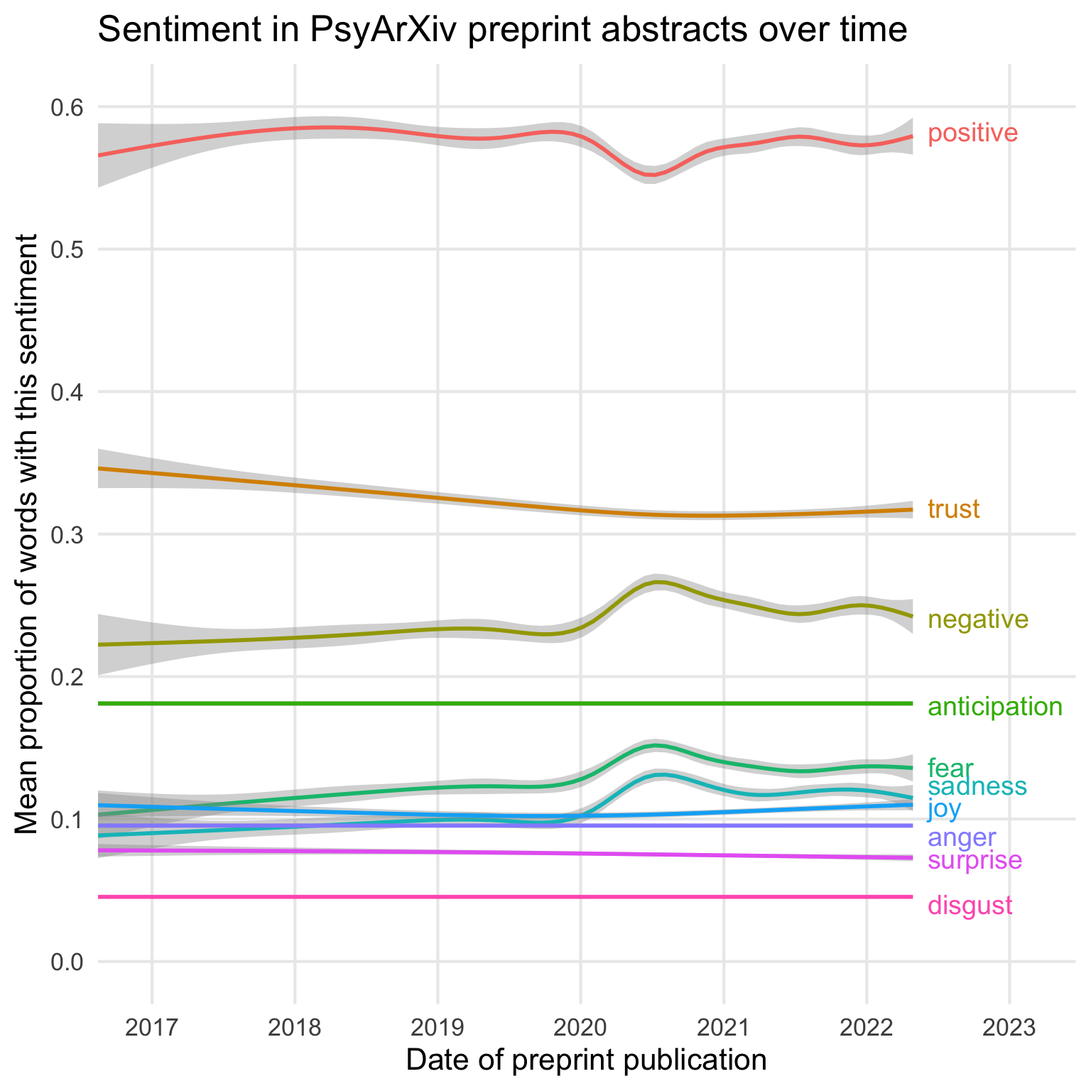
29.3.2 Text labels

Hide the legend and add text annotation to the end of the pot with geom_text(). Make sure to use a dataset with only one row per sentiment, or it will try to print the labels thousands of times. You have to set the x value as a datetime, so use now() and add or subtract time.

Code

ggplot(sentiment, aes(x = pub_dt, y = value, color = sentiment)) +
  geom_smooth() +
  geom_text(data = s_order, 
            aes(y = v, label = sentiment), 
            x = now() + months(1), 
            hjust = 0, size = 5) +
  scale_x_datetime(date_breaks = "1 year",
                   date_labels = "%Y",
                   expand = expansion(mult = c(0, .2))) +
  scale_y_continuous(breaks = seq(0, 1, .1)) +
  coord_cartesian(ylim = c(0, 0.6)) +
  labs(x = "Date of preprint publication",
       y = "Mean proportion of words with this sentiment",
       title = "Sentiment in PsyArXiv preprint abstracts over time",
       cation = "Data from OSF.io API") +
  theme(legend.position = "none",
        panel.grid.minor = element_blank())